Analysis

56 - City Centerline and OTP

Coverage: 2019-01 to 2025-11 (from otp_monthly).

Built 2026-06-15 11:52 UTC · Commit e5cf673

Page Navigation

Analysis Navigation

Data Provenance

flowchart LR
  56_city_centerline_otp(["56 - City Centerline and OTP"])
  t_otp_monthly[("otp_monthly")] --> 56_city_centerline_otp
  01_data_ingestion[["Data Ingestion"]] --> t_otp_monthly
  u1_01_data_ingestion[/"data/routes_by_month.csv"/] --> 01_data_ingestion
  u2_01_data_ingestion[/"data/PRT_Current_Routes_Full_System_de0e48fcbed24ebc8b0d933e47b56682.csv"/] --> 01_data_ingestion
  u3_01_data_ingestion[/"data/Transit_stops_(current)_by_route_e040ee029227468ebf9d217402a82fa9.csv"/] --> 01_data_ingestion
  u4_01_data_ingestion[/"data/PRT_Stop_Reference_Lookup_Table.csv"/] --> 01_data_ingestion
  u5_01_data_ingestion[/"data/average-ridership/12bb84ed-397e-435c-8d1b-8ce543108698.csv"/] --> 01_data_ingestion
  t_route_road_city[("route_road_city")] --> 56_city_centerline_otp
  13_city_centerline[["City Centerline Overlay ETL"]] --> t_route_road_city
  u1_13_city_centerline[/"data/pgh-centerline/centerline_raw.geojson"/] --> 13_city_centerline
  u2_13_city_centerline[/"data/GTFS/shapes.txt"/] --> 13_city_centerline
  u3_13_city_centerline[/"data/GTFS/trips.txt"/] --> 13_city_centerline
  u4_13_city_centerline{"City of Pittsburgh Street Centerline (ArcGIS Hub)"} --> 13_city_centerline
  t_route_road_class[("route_road_class")] --> 56_city_centerline_otp
  12_road_classification[["Road Classification Overlay ETL"]] --> t_route_road_class
  u1_12_road_classification[/"data/penndot-roadclass/roadwaysegments.json"/] --> 12_road_classification
  u2_12_road_classification[/"data/penndot-roadclass/roadwayadmin.json"/] --> 12_road_classification
  u3_12_road_classification[/"data/GTFS/shapes.txt"/] --> 12_road_classification
  u4_12_road_classification[/"data/GTFS/trips.txt"/] --> 12_road_classification
  u5_12_road_classification{"PennDOT ArcGIS Roadway Segments Layer (RMSSEG)"} --> 12_road_classification
  u6_12_road_classification{"PennDOT ArcGIS Roadway Admin Layer"} --> 12_road_classification
  t_route_stops[("route_stops")] --> 56_city_centerline_otp
  01_data_ingestion[["Data Ingestion"]] --> t_route_stops
  t_stops[("stops")] --> 56_city_centerline_otp
  01_data_ingestion[["Data Ingestion"]] --> t_stops
  t_routes[("routes")] --> 56_city_centerline_otp
  01_data_ingestion[["Data Ingestion"]] --> t_routes
  d1_56_city_centerline_otp(("analyses/55_road_classification_otp (lib)")) --> 56_city_centerline_otp
  classDef page fill:#dbeafe,stroke:#1d4ed8,color:#1e3a8a,stroke-width:2px;
  classDef table fill:#ecfeff,stroke:#0e7490,color:#164e63;
  classDef dep fill:#fff7ed,stroke:#c2410c,color:#7c2d12,stroke-dasharray: 4 2;
  classDef file fill:#eef2ff,stroke:#6366f1,color:#3730a3;
  classDef api fill:#f0fdf4,stroke:#16a34a,color:#14532d;
  classDef pipeline fill:#f5f3ff,stroke:#7c3aed,color:#4c1d95;
  class 56_city_centerline_otp page;
  class t_otp_monthly,t_route_road_city,t_route_road_class,t_route_stops,t_routes,t_stops table;
  class d1_56_city_centerline_otp dep;
  class u1_01_data_ingestion,u1_12_road_classification,u1_13_city_centerline,u2_01_data_ingestion,u2_12_road_classification,u2_13_city_centerline,u3_01_data_ingestion,u3_12_road_classification,u3_13_city_centerline,u4_01_data_ingestion,u4_12_road_classification,u5_01_data_ingestion file;
  class u4_13_city_centerline,u5_12_road_classification,u6_12_road_classification api;
  class 01_data_ingestion,12_road_classification,13_city_centerline pipeline;

Findings

Findings: City Centerline and OTP

Summary

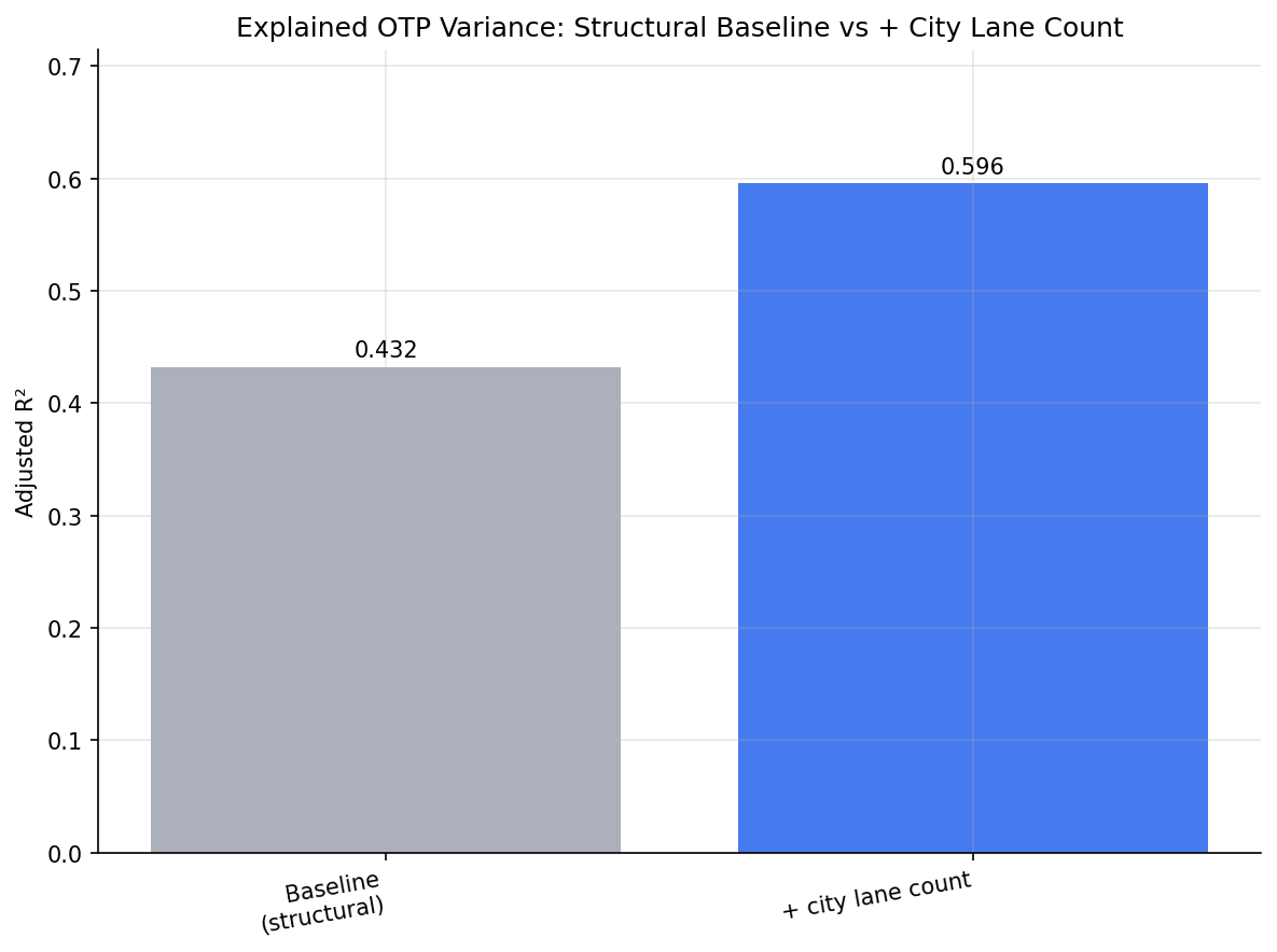
Analysis 55 found that buses on wider, multi-lane roads run late more often, using PennDOT's state-road inventory. This analysis re-tests that finding with a fully independent dataset -- the City of Pittsburgh street centerline, which counts lanes on the entire city street network, local streets included -- and the result holds almost exactly. City-network lane count correlates with OTP at r = -0.44 (vs PennDOT's -0.47), and adding it to the structural baseline lifts explained variance from 43% to 60% (a +0.16 jump in adjusted R², F = 29.4, p < 0.0001). Two lane-count measures built from different agencies' data, by different methods, point to the same conclusion: road width is a real, robust correlate of on-time performance, not an artifact of which roads PennDOT happens to inventory.

Key Numbers

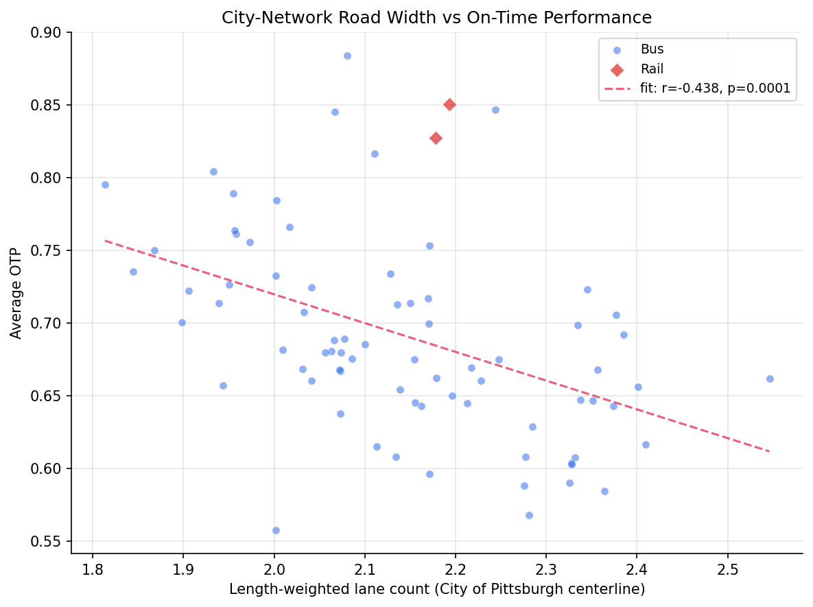
  • City lane count vs OTP: r = -0.438 (p = 0.0001, n = 77 routes). Analysis 55 PennDOT: r = -0.470.
  • Regression gain: adjusted R² 0.432 -> 0.596 (+0.164) when city lane count is added to the 6-feature structural baseline. Nested F = 29.4, p < 0.0001.
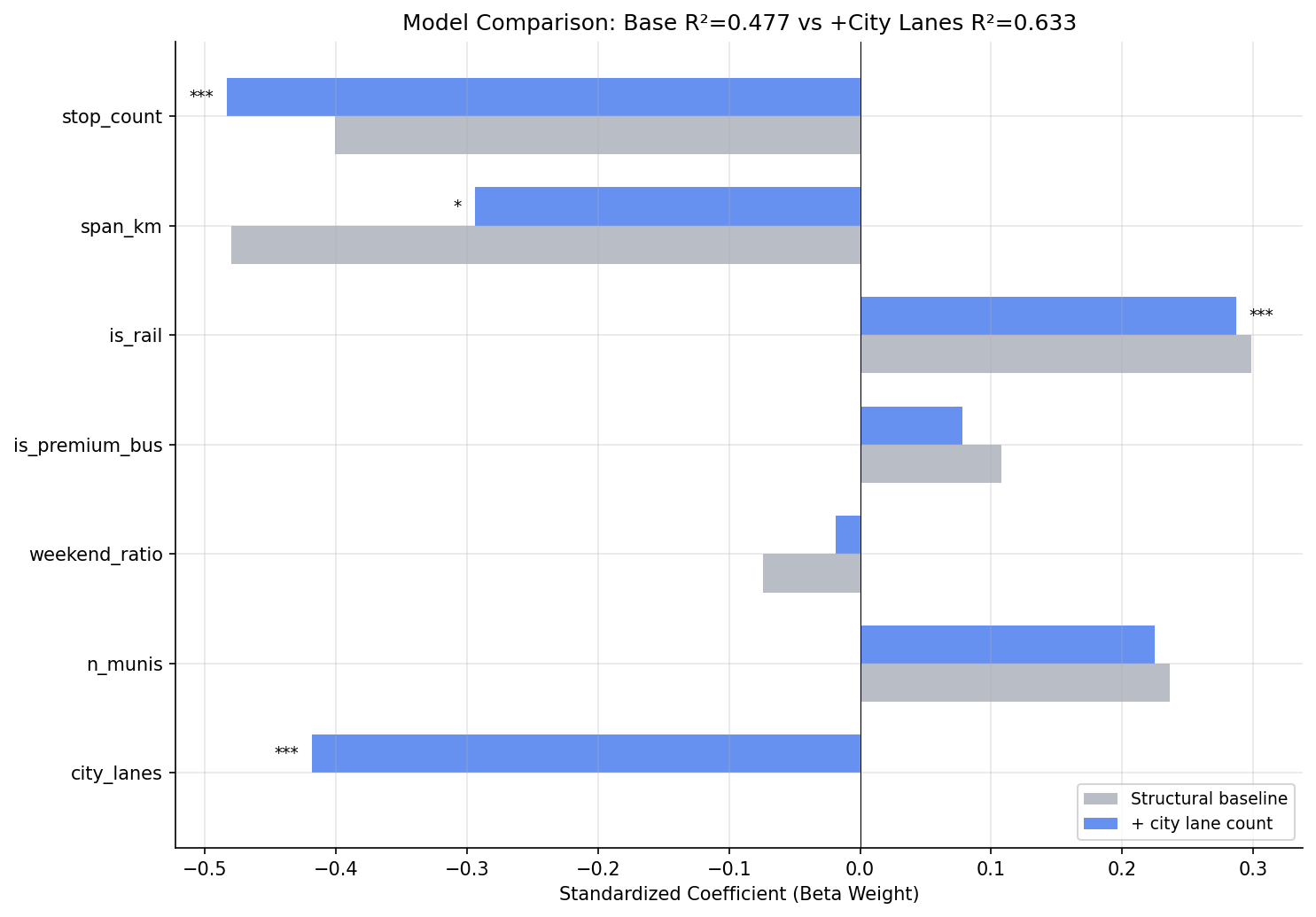
  • City lane count beta weight: -0.418 (p < 0.0001) -- the largest standardized effect in the augmented model, comparable to stop count (-0.483) and span (-0.294).
  • VIF for city lane count = 1.12 -- essentially no collinearity with the structural features; it carries independent information.
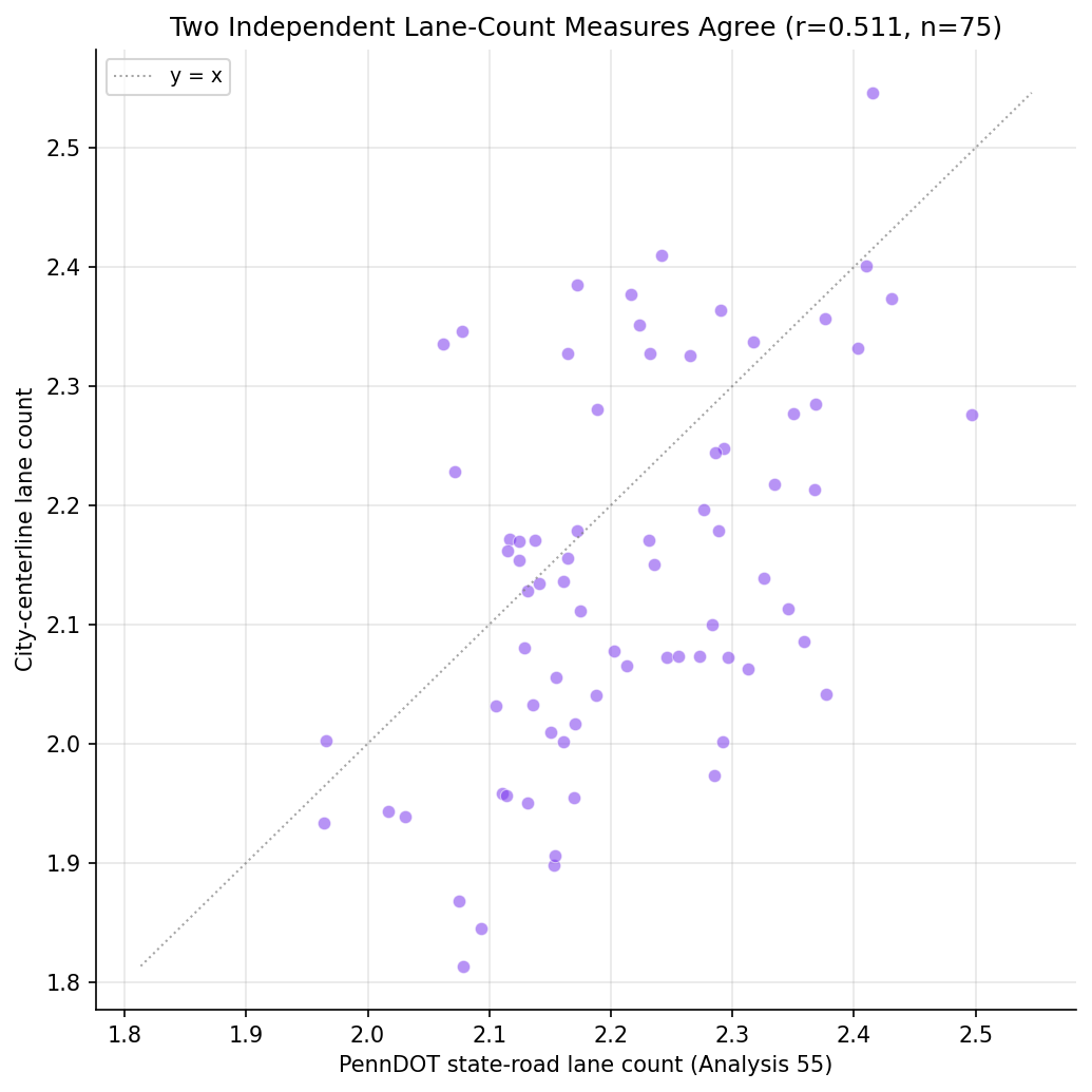
  • Two measures agree: city vs PennDOT lane count correlate at r = +0.511 (n = 75); means 2.14 (city) vs 2.21 (PennDOT) lanes.
  • Bus-only: adjusted R² 0.365 -> 0.549 when city lane count is added (F = 29.1, p < 0.0001).
  • Coverage: 77 of 89 city-matched routes have match_rate >= 0.3; median within-city coverage 66%.

Observations

  • The lane-count finding replicates on an independent dataset. The whole point of this analysis was to check whether Analysis 55's lane-count effect was an artifact of PennDOT's state-road selection. It is not: a different agency's inventory, covering a broader set of streets (including local roads PennDOT omits), produces a near-identical correlation and an even larger single-predictor R² gain.
  • The two lane-count measures are related but not identical (r = +0.51), yet both predict OTP about equally. If the effect were a measurement artifact, the two differently-built measures would not agree this consistently on direction and magnitude. Their partial agreement (city lanes fold in local 1-2 lane streets, lowering the mean slightly from 2.21 to 2.14) is what we would expect from two honest measures of the same underlying road width.
  • Coverage expansion turned out modest. The original phase-2 hope was that the city centerline would fill in routes PennDOT misses. In practice it added only ~2 such routes: city routes spend roughly half their length outside Pittsburgh limits (median within-city coverage 66%), where the centerline does not reach. The analysis's value is robustness, not coverage.
  • One-way share and limited-access (freeway) share show no association with OTP (r = +0.03 and +0.01, both n.s.). Lane count alone carries the road-width signal, consistent with Analysis 55, where lane count dominated functional class and posted speed.

Caveats

  • Area-level (ecological) association. This is a route-level relationship between the roads a route runs along and its aggregate OTP. It does not establish that any individual trip is late because of a wide road; lane count co-varies with downtown/arterial operating environments, signal density, and traffic that are not all separately controlled here.
  • City-limits coverage only. The centerline covers City of Pittsburgh streets, so suburban portions of routes are unmeasured. Routes are included only when at least 30% of their shape matches a city street; 12 low-coverage routes were excluded. The lane metric describes each route's within-city roads.
  • CFCC functional class is not usable here. The dataset's Census Feature Class Codes are largely degenerate (A3* lumps ~88% of streets), so functional class was not used as a predictor. Only lane count and the A1* limited-access flag were derived.
  • Lane count 0/null treated as missing. ~8% of segments lack a usable lane count; these are dropped from the length-weighted mean rather than counted as zero-lane roads.
  • Not a causal or independent corroboration of magnitude. Because city and PennDOT lane counts are correlated (r = 0.51), this is a robustness check on the existence and direction of the effect, not a fully independent second estimate of its size.

Validation

Data inputs

  1. Data source verified. route_road_city columns checked against prt_otp_analysis.common.schemas.ROUTE_ROAD_CITY and validated at load (validate(..., subset=True)). Centerline fields (no_lanes, cfcc, oneway) confirmed against the live ArcGIS service before building (see data/pgh-centerline/SOURCE.md).
  2. Geographic/temporal scope matches. OTP averaged over routes with 12+ months; lane metrics matched to the same GTFS route shapes used throughout the project (30 m buffer, identical KDTree machinery as Analyses 27/55). City-limits coverage limitation documented.
  3. Null/missing handling. Lane count 0 and null treated as missing in the length-weighted mean (not as zero-lane roads). Routes with match_rate < 0.3 excluded, not imputed.

Results plausibility

  1. Aggregates sanity-checked. Mean lane count 2.14 (city) is consistent with a predominantly 1-2-lane urban street network and sits just below PennDOT's 2.21 (state roads skew wider), exactly as expected when local streets are folded in.
  2. Surprising results investigated. The result is not surprising -- it confirms Analysis 55 with an independent dataset, which was the goal. The direction (more lanes -> lower OTP) matches the established finding.
  3. Direction of effects checked. Negative lane-count -> OTP slope reproduces Analysis 55; rail dummy positive; stop count and span negative -- all consistent with prior structural models.

Statistical diagnostics

  1. Multicollinearity checked. VIF reported for all predictors; max is span_km at 3.66. City lane count VIF = 1.12. No predictor exceeds 5.
  2. Small-sample routes flagged. Minimum 12 months of OTP and match_rate >= 0.3 enforced; n = 77 routes (75 bus, 2 rail). The 2-route rail subset is noted, not over-interpreted.
  3. Ecological framing. Results described as route/area-level associations throughout; no individual-trip causal claim is made.

Output
Methods

Methods: City Centerline and OTP

Question

Analysis 55 found that lane count is the strongest road-type predictor of OTP (r = -0.47), but it was computed only over PennDOT state roads -- the major, arterial portion of each route. Two concerns follow: (1) is the lane-count signal a real road-width effect, or an artifact of which segments PennDOT happens to inventory? (2) does it hold on the broader street network, including the local 1-2 lane streets that state-road data omits? This analysis answers both by recomputing route lane count from a fully independent dataset -- the City of Pittsburgh street centerline -- and re-testing it against OTP.

This is primarily a robustness / cross-validation analysis, not a coverage-expansion one: the city centerline matches almost the same routes PennDOT does (the centerline is city-limits-only, so suburban route segments are uncovered), but it measures lane count a completely different way, from a different agency's inventory of a broader set of streets.

Approach

  • Build route_road_city (pipeline step 13): for each route, the length-weighted mean lane count of city street segments within 30 m of its GTFS shape, plus one-way share and limited-access (freeway, CFCC A1*) share. Lane count 0/null is treated as missing. Match rate records the within-buffer (≈ within-city) fraction of the route.
  • Include routes with 12+ months of OTP and route_road_city.match_rate >= 0.3.
  • Bivariate: correlate city-network lane count with OTP, and compare against Analysis 55's PennDOT lane-count correlation.
  • Head-to-head: for routes matched by both datasets, compare the city vs PennDOT lane count (means and Pearson r) to show they are related but distinct measures.
  • Regression: replicate the Analysis 18/55 six-feature structural OLS baseline on the city-matched sample, then add city lane count and test the improvement with a nested F-test. Compute VIF for the augmented model and flag any predictor with VIF > 5.
  • Report one-way share and limited-access share descriptively (Pearson r with OTP).
  • Repeat the base-vs-lanes comparison on the bus-only subset.

The CFCC functional-class codes in this dataset are largely degenerate (A3* lumps ~88% of streets), so functional class is not used as a predictor; lane count carries the road-width signal, consistent with Analysis 55 where lane count dominated.

All regression helpers (compute_span, fit_ols, compute_vif, f_test_nested) are replicated locally so the analysis does not import from Analysis 18/55 (analyses must be independent).

Data

Name Description Source
otp_monthly route_id, month, otp (averaged to route level, 12+ months required) prt.db table
route_road_city route_id, weighted_lanes, oneway_share, limited_access_share, match_rate (built by road_overlay_city.py, pipeline step 13) prt.db table
route_road_class route_id, weighted_lanes (PennDOT, for head-to-head comparison) prt.db table
route_stops stop counts, trip frequencies prt.db table
stops lat, lon for geographic span; muni for municipality count prt.db table
routes route_id, mode for subtype classification prt.db table

Inclusion: routes with 12+ months of OTP and route_road_city.match_rate >= 0.3. Lane count is length-weighted over the City of Pittsburgh centerline segments within 30 m of the route's GTFS shape. Because the centerline is city-limits-only, routes that run into the suburbs are only partially covered; the match rate quantifies the covered share.

Output

  • output/model_comparison.csv -- regression results (base vs + city lanes, bus subset)
  • output/vif_table.csv -- VIF values for the augmented model
  • output/route_road_city_summary.csv -- per-route city vs PennDOT lane metrics with OTP
  • output/city_lanes_vs_otp.png -- bivariate scatter of city lane count vs OTP
  • output/city_vs_penndot_lanes.png -- city vs PennDOT lane count agreement scatter
  • output/r2_progression.png -- adjusted R² baseline vs + city lanes
  • output/coefficient_comparison.png -- beta-weight comparison, base vs augmented model

Source Code

"""Analysis 56: Cross-validate the Analysis 55 lane-count -> OTP finding using the
independent City of Pittsburgh street-centerline lane counts (which include local streets)."""

import math

import numpy as np
import polars as pl
from scipy import stats

from prt_otp_analysis.common import (
    analysis_dir,
    classify_bus_route,
    correlate,
    phase,
    query_to_polars,
    run_analysis,
    save_chart,
    save_csv,
    setup_plotting,
)
from prt_otp_analysis.common.schemas import ROUTE_ROAD_CITY, validate

OUT = analysis_dir(__file__)

MIN_MONTHS = 12
MIN_MATCH_RATE = 0.3


# ---------------------------------------------------------------------------
# Helpers (replicated from Analysis 18/55 to keep analyses independent)
# ---------------------------------------------------------------------------

def haversine_km(lat1: float, lon1: float, lat2: float, lon2: float) -> float:
    """Return the great-circle distance in km between two lat/lon points."""
    R = 6371.0
    dlat = math.radians(lat2 - lat1)
    dlon = math.radians(lon2 - lon1)
    a = (math.sin(dlat / 2) ** 2
         + math.cos(math.radians(lat1)) * math.cos(math.radians(lat2))
         * math.sin(dlon / 2) ** 2)
    return R * 2 * math.atan2(math.sqrt(a), math.sqrt(1 - a))


def compute_span(lats: list[float], lons: list[float]) -> float:
    """Return the max pairwise haversine distance (km) among a set of points."""
    max_dist = 0.0
    n = len(lats)
    for i in range(n):
        for j in range(i + 1, n):
            d = haversine_km(lats[i], lons[i], lats[j], lons[j])
            if d > max_dist:
                max_dist = d
    return max_dist


def compute_vif(X_raw: np.ndarray, feature_names: list[str]) -> dict[str, float]:
    """Compute Variance Inflation Factor for each predictor."""
    n, k = X_raw.shape
    vifs = {}
    for j in range(k):
        y_j = X_raw[:, j]
        X_other = np.delete(X_raw, j, axis=1)
        X_other = np.column_stack([np.ones(n), X_other])
        beta, _, _, _ = np.linalg.lstsq(X_other, y_j, rcond=None)
        y_hat = X_other @ beta
        ss_res = np.sum((y_j - y_hat) ** 2)
        ss_tot = np.sum((y_j - np.mean(y_j)) ** 2)
        r2_j = 1 - ss_res / ss_tot if ss_tot > 0 else 0.0
        vifs[feature_names[j]] = 1.0 / (1.0 - r2_j) if r2_j < 1.0 else float("inf")
    return vifs


def fit_ols(y: np.ndarray, X_raw: np.ndarray, feature_names: list[str]) -> dict:
    """Fit OLS regression and return results dict."""
    n, k = X_raw.shape
    X = np.column_stack([np.ones(n), X_raw])

    beta, _, _, _ = np.linalg.lstsq(X, y, rcond=None)
    y_hat = X @ beta
    residuals = y - y_hat

    ss_res = np.sum(residuals ** 2)
    ss_tot = np.sum((y - np.mean(y)) ** 2)
    r_squared = 1 - ss_res / ss_tot
    adj_r_squared = 1 - (1 - r_squared) * (n - 1) / (n - k - 1)
    mse = ss_res / (n - k - 1)

    XtX_inv = np.linalg.pinv(X.T @ X)
    se = np.sqrt(np.diag(XtX_inv) * mse)
    t_vals = beta / se
    p_vals = [2 * (1 - stats.t.cdf(abs(t), df=n - k - 1)) for t in t_vals]

    x_stds = np.std(X_raw, axis=0, ddof=1)
    y_std = np.std(y, ddof=1)
    beta_weights = beta[1:] * x_stds / y_std

    return {
        "r_squared": r_squared,
        "adj_r_squared": adj_r_squared,
        "ss_res": ss_res,
        "n": n,
        "k": k,
        "features": ["intercept"] + feature_names,
        "coefficients": beta.tolist(),
        "std_errors": se.tolist(),
        "t_values": t_vals.tolist(),
        "p_values": p_vals,
        "beta_weights": [None] + beta_weights.tolist(),
        "y_hat": y_hat,
        "residuals": residuals,
    }


def f_test_nested(base: dict, full: dict) -> tuple[float, float]:
    """F-test comparing nested models. Returns (F_stat, p_value)."""
    k_diff = full["k"] - base["k"]
    n = full["n"]
    f_stat = ((base["ss_res"] - full["ss_res"]) / k_diff) / (full["ss_res"] / (n - full["k"] - 1))
    f_p = 1 - stats.f.cdf(f_stat, k_diff, n - full["k"] - 1)
    return f_stat, f_p


def print_model(results: dict, label: str) -> None:
    """Print formatted model results."""
    print(f"\n  {label}:")
    print(f"  R2 = {results['r_squared']:.4f}, Adj R2 = {results['adj_r_squared']:.4f}, "
          f"n = {results['n']}, k = {results['k']}")
    print(f"  {'Feature':<20s} {'Coeff':>10s} {'Std Err':>10s} {'p-value':>10s} {'Beta':>10s}")
    print(f"  {'-'*60}")
    for i, feat in enumerate(results["features"]):
        coeff = results["coefficients"][i]
        se = results["std_errors"][i]
        p = results["p_values"][i]
        beta = results["beta_weights"][i]
        beta_str = f"{beta:>10.4f}" if beta is not None else f"{'--':>10s}"
        sig = "***" if p < 0.001 else "**" if p < 0.01 else "*" if p < 0.05 else ""
        print(f"  {feat:<20s} {coeff:>10.6f} {se:>10.6f} {p:>10.4f} {beta_str} {sig}")


# ---------------------------------------------------------------------------
# Data loading
# ---------------------------------------------------------------------------

def load_features() -> pl.DataFrame:
    """Assemble structural features + city-centerline lane data for the regression."""
    avg_otp_df = query_to_polars(f"""
        SELECT o.route_id, r.route_name, r.mode,
               AVG(o.otp) AS avg_otp, COUNT(*) AS months
        FROM otp_monthly o
        JOIN routes r ON o.route_id = r.route_id
        GROUP BY o.route_id
        HAVING COUNT(*) >= {MIN_MONTHS}
    """)

    stop_counts_df = query_to_polars("""
        SELECT route_id, COUNT(DISTINCT stop_id) AS stop_count
        FROM route_stops GROUP BY route_id
    """)
    trips_df = query_to_polars("""
        SELECT route_id,
               MAX(trips_wd) AS max_wd,
               MAX(trips_sa) AS max_sa,
               MAX(trips_su) AS max_su
        FROM route_stops GROUP BY route_id
    """)
    munis_df = query_to_polars("""
        SELECT rs.route_id, COUNT(DISTINCT s.muni) AS n_munis
        FROM route_stops rs
        JOIN stops s ON rs.stop_id = s.stop_id
        WHERE s.muni IS NOT NULL AND s.muni != '0'
        GROUP BY rs.route_id
    """)
    stops_by_route_df = query_to_polars("""
        SELECT rs.route_id, s.lat, s.lon
        FROM route_stops rs
        JOIN stops s ON rs.stop_id = s.stop_id
        WHERE s.lat IS NOT NULL AND s.lon IS NOT NULL
    """)
    spans = []
    for route_id in stops_by_route_df["route_id"].unique().sort().to_list():
        subset = stops_by_route_df.filter(pl.col("route_id") == route_id)
        span_km = compute_span(subset["lat"].to_list(), subset["lon"].to_list())
        spans.append({"route_id": route_id, "span_km": span_km})
    span_df = pl.DataFrame(spans)

    city_df = query_to_polars("""
        SELECT route_id, weighted_lanes AS city_lanes, oneway_share,
               limited_access_share, match_rate, n_segments, total_length_ft
        FROM route_road_city
    """)
    validate(
        city_df.rename({"city_lanes": "weighted_lanes"}),
        ROUTE_ROAD_CITY, subset=True,
    )

    # PennDOT lanes for head-to-head comparison (renamed to avoid collision).
    penndot_df = query_to_polars("""
        SELECT route_id, weighted_lanes AS penndot_lanes, match_rate AS penndot_match_rate
        FROM route_road_class
    """)

    df = avg_otp_df
    df = df.join(stop_counts_df, on="route_id", how="left")
    df = df.join(trips_df, on="route_id", how="left")
    df = df.join(munis_df, on="route_id", how="left")
    df = df.join(span_df, on="route_id", how="left")
    df = df.join(city_df, on="route_id", how="inner")
    df = df.join(penndot_df, on="route_id", how="left")

    df = df.with_columns(
        pl.when(pl.col("max_wd") > 0)
        .then((pl.col("max_sa") + pl.col("max_su")) / (2.0 * pl.col("max_wd")))
        .otherwise(0.0)
        .alias("weekend_ratio"),
    )
    df = df.with_columns(
        pl.when(pl.col("mode") == "RAIL").then(1.0).otherwise(0.0).alias("is_rail"),
    )
    df = df.with_columns(
        pl.when(pl.col("mode") == "BUS")
        .then(pl.col("route_id").map_elements(classify_bus_route, return_dtype=pl.Utf8))
        .otherwise(pl.lit("non_bus"))
        .alias("bus_subtype"),
    )
    df = df.with_columns(
        pl.when(pl.col("bus_subtype").is_in(["busway", "flyer", "express", "limited"]))
        .then(1.0)
        .otherwise(0.0)
        .alias("is_premium_bus"),
    )

    df = df.drop_nulls(subset=["stop_count", "span_km", "weekend_ratio", "n_munis", "city_lanes"])
    return df


# ---------------------------------------------------------------------------
# Charts
# ---------------------------------------------------------------------------

def make_city_lanes_scatter(df: pl.DataFrame) -> None:
    """Bivariate scatter: city-network lane count vs OTP."""
    plt = setup_plotting()
    fig, ax = plt.subplots(figsize=(8, 6))

    lanes = df["city_lanes"].to_numpy()
    otp = df["avg_otp"].to_numpy()
    modes = df["mode"].to_list()
    bus_mask = np.array([m == "BUS" for m in modes])
    rail_mask = ~bus_mask

    ax.scatter(lanes[bus_mask], otp[bus_mask], alpha=0.5, s=30, color="#2563eb",
               edgecolors="white", linewidth=0.5, label="Bus", zorder=2)
    if np.any(rail_mask):
        ax.scatter(lanes[rail_mask], otp[rail_mask], alpha=0.7, s=50, color="#dc2626",
                   marker="D", edgecolors="white", linewidth=0.5, label="Rail", zorder=3)

    slope, intercept, r, p, _ = stats.linregress(lanes, otp)
    x_line = np.array([lanes.min(), lanes.max()])
    ax.plot(x_line, slope * x_line + intercept, color="#e11d48", linewidth=1.5,
            linestyle="--", alpha=0.7, label=f"fit: r={r:.3f}, p={p:.4f}")

    ax.set_xlabel("Length-weighted lane count (City of Pittsburgh centerline)")
    ax.set_ylabel("Average OTP")
    ax.set_title("City-Network Road Width vs On-Time Performance")
    ax.legend(fontsize=9)
    save_chart(fig, OUT / "city_lanes_vs_otp.png")


def make_city_vs_penndot(df: pl.DataFrame) -> None:
    """Scatter of city-centerline lane count vs PennDOT lane count for shared routes."""
    plt = setup_plotting()
    fig, ax = plt.subplots(figsize=(7, 7))

    sub = df.drop_nulls(subset=["penndot_lanes"]).filter(
        pl.col("penndot_match_rate") >= MIN_MATCH_RATE
    )
    city = sub["city_lanes"].to_numpy()
    pdot = sub["penndot_lanes"].to_numpy()

    ax.scatter(pdot, city, alpha=0.55, s=35, color="#7c3aed",
               edgecolors="white", linewidth=0.5, zorder=2)
    lo = min(city.min(), pdot.min())
    hi = max(city.max(), pdot.max())
    ax.plot([lo, hi], [lo, hi], color="gray", linewidth=1.0, linestyle=":",
            alpha=0.7, label="y = x")
    r, p = stats.pearsonr(pdot, city)
    ax.set_xlabel("PennDOT state-road lane count (Analysis 55)")
    ax.set_ylabel("City-centerline lane count")
    ax.set_title(f"Two Independent Lane-Count Measures Agree (r={r:.3f}, n={len(sub)})")
    ax.legend(fontsize=9)
    save_chart(fig, OUT / "city_vs_penndot_lanes.png")


def make_r2_progression(model_specs: list[tuple[str, dict]]) -> None:
    """Bar chart of adjusted R^2 across the nested models (same sample)."""
    plt = setup_plotting()
    fig, ax = plt.subplots(figsize=(8, 6))

    labels = [label for label, _ in model_specs]
    adj_r2 = [m["adj_r_squared"] for _, m in model_specs]
    colors = ["#9ca3af", "#2563eb"][: len(labels)]

    bars = ax.bar(labels, adj_r2, color=colors, alpha=0.85)
    for bar, val in zip(bars, adj_r2):
        ax.text(bar.get_x() + bar.get_width() / 2, val + 0.005, f"{val:.3f}",
                ha="center", va="bottom", fontsize=10)

    ax.set_ylabel("Adjusted R²")
    ax.set_title("Explained OTP Variance: Structural Baseline vs + City Lane Count")
    ax.set_ylim(0, max(adj_r2) * 1.2)
    plt.xticks(rotation=10, ha="right")
    save_chart(fig, OUT / "r2_progression.png")


def make_coefficient_chart(base: dict, full: dict) -> None:
    """Compare standardized coefficients between base and augmented models."""
    plt = setup_plotting()
    fig, ax = plt.subplots(figsize=(10, 7))

    full_feats = full["features"][1:]
    base_betas = {f: b for f, b in zip(base["features"][1:], base["beta_weights"][1:])}
    full_betas = {f: b for f, b in zip(full_feats, full["beta_weights"][1:])}
    full_pvals = {f: p for f, p in zip(full_feats, full["p_values"][1:])}

    y_pos = np.arange(len(full_feats))
    width = 0.35
    base_vals = [base_betas.get(f, 0.0) for f in full_feats]
    full_vals = [full_betas[f] for f in full_feats]

    ax.barh(y_pos + width / 2, base_vals, width, label="Structural baseline",
            color="#9ca3af", alpha=0.7)
    ax.barh(y_pos - width / 2, full_vals, width, label="+ city lane count",
            color="#2563eb", alpha=0.7)

    for i, f in enumerate(full_feats):
        p = full_pvals[f]
        marker = "***" if p < 0.001 else "**" if p < 0.01 else "*" if p < 0.05 else ""
        val = full_vals[i]
        ax.text(val + 0.01 if val >= 0 else val - 0.01, i - width / 2, marker,
                ha="left" if val >= 0 else "right", va="center", fontsize=9)

    ax.set_yticks(y_pos)
    ax.set_yticklabels(full_feats)
    ax.axvline(0, color="black", linewidth=0.5)
    ax.set_xlabel("Standardized Coefficient (Beta Weight)")
    ax.set_title(f"Model Comparison: Base R²={base['r_squared']:.3f} vs "
                 f"+City Lanes R²={full['r_squared']:.3f}")
    ax.legend(loc="lower right", fontsize=9)
    ax.invert_yaxis()
    save_chart(fig, OUT / "coefficient_comparison.png")


# ---------------------------------------------------------------------------
# Main
# ---------------------------------------------------------------------------

@run_analysis(56, "City Centerline and OTP")
def main() -> None:
    """Entry point: load features, cross-validate lane->OTP, fit nested models, chart."""

    with phase("Loading and assembling features"):
        df_all = load_features()
        df = df_all.filter(pl.col("match_rate") >= MIN_MATCH_RATE)
        excluded = df_all.filter(pl.col("match_rate") < MIN_MATCH_RATE)
        n_rail = len(df.filter(pl.col("is_rail") == 1.0))
        n_bus = len(df.filter(pl.col("mode") == "BUS"))
        print(f"  {len(df)} routes after match_rate >= {MIN_MATCH_RATE} filter "
              f"({n_bus} BUS, {n_rail} RAIL)")
        if len(excluded) > 0:
            print(f"  Excluded ({len(excluded)}, low city coverage): "
                  + ", ".join(excluded.sort("match_rate")["route_id"].to_list()))
        print(f"\n  City lane count range: {df['city_lanes'].min():.2f} -- "
              f"{df['city_lanes'].max():.2f} (mean {df['city_lanes'].mean():.2f})")
        print(f"  Median city match rate: {df['match_rate'].median():.1%}")

    y = df["avg_otp"].to_numpy()

    # --- Bivariate cross-validation against Analysis 55 ---
    with phase("Bivariate: city lane count vs OTP (cross-validation)"):
        corr = correlate(df, "city_lanes", "avg_otp")
        print(f"  City lanes vs OTP:    r = {corr['pearson_r']:+.3f}, "
              f"p = {corr['pearson_p']:.4f} (n={len(df)})")
        print("  Analysis 55 PennDOT:  r = -0.470 (state roads only)")
        for feat in ["oneway_share", "limited_access_share"]:
            sub = df.drop_nulls(subset=[feat])
            c = correlate(sub, feat, "avg_otp")
            sig = "*" if c["pearson_p"] < 0.05 else ""
            print(f"  {feat:<20s} r = {c['pearson_r']:+.3f}, "
                  f"p = {c['pearson_p']:.4f} (n={len(sub)}) {sig}")

    # --- Head-to-head: city vs PennDOT lanes ---
    both_df = df.drop_nulls(subset=["penndot_lanes"]).filter(
        pl.col("penndot_match_rate") >= MIN_MATCH_RATE
    )
    with phase(f"Head-to-head city vs PennDOT lanes (n={len(both_df)})"):
        cl = both_df["city_lanes"].to_numpy()
        pdot = both_df["penndot_lanes"].to_numpy()
        r_cp, p_cp = stats.pearsonr(cl, pdot)
        print(f"  Mean lanes -- city: {cl.mean():.2f}, PennDOT: {pdot.mean():.2f}")
        print(f"  Correlation between the two measures: r = {r_cp:+.3f}, p = {p_cp:.4f}")
        print("  (Two independently-built measures agreeing => real road-width signal.)")

    base_features = ["stop_count", "span_km", "is_rail", "is_premium_bus",
                     "weekend_ratio", "n_munis"]

    # --- Model 1: structural baseline ---
    X_base = np.column_stack([df[f].to_numpy().astype(float) for f in base_features])
    with phase("Fitting structural baseline (6 features)"):
        base = fit_ols(y, X_base, base_features)
        print_model(base, "Structural baseline (6 features)")

    # --- Model 2: + city lane count ---
    full_features = base_features + ["city_lanes"]
    X_full = np.column_stack([df[f].to_numpy().astype(float) for f in full_features])
    with phase("Fitting + city lane count"):
        full = fit_ols(y, X_full, full_features)
        print_model(full, "Base + city lane count")
        f_stat, f_p = f_test_nested(base, full)
        print(f"\n  F-test for city lane count: F = {f_stat:.3f}, p = {f_p:.4f}")
        print(f"  Adj R2: {base['adj_r_squared']:.4f} -> {full['adj_r_squared']:.4f} "
              f"(+{full['adj_r_squared'] - base['adj_r_squared']:.4f})")
        if f_p < 0.05:
            print("  => City lane count IS significant after controlling for structural features.")
        else:
            print("  => City lane count is NOT significant after structural controls.")

    # --- VIF ---
    with phase("VIF (augmented model)"):
        vifs = compute_vif(X_full, full_features)
        for feat, vif in vifs.items():
            flag = " ** HIGH" if vif > 5 else ""
            print(f"  {feat:<20s} VIF = {vif:.2f}{flag}")

    # --- Bus-only subgroup ---
    bus_df = df.filter(pl.col("mode") == "BUS")
    with phase(f"Fitting bus-only models ({len(bus_df)} routes)"):
        y_bus = bus_df["avg_otp"].to_numpy()
        bus_base_feats = ["stop_count", "span_km", "is_premium_bus", "weekend_ratio", "n_munis"]
        bus_full_feats = bus_base_feats + ["city_lanes"]
        X_bus_base = np.column_stack([bus_df[f].to_numpy().astype(float) for f in bus_base_feats])
        X_bus_full = np.column_stack([bus_df[f].to_numpy().astype(float) for f in bus_full_feats])
        bus_base = fit_ols(y_bus, X_bus_base, bus_base_feats)
        bus_full = fit_ols(y_bus, X_bus_full, bus_full_feats)
        f_b, fp_b = f_test_nested(bus_base, bus_full)
        print(f"  Bus-only F-test for city lane count: F = {f_b:.3f}, p = {fp_b:.4f}")
        print(f"  Adj R2: {bus_base['adj_r_squared']:.4f} -> {bus_full['adj_r_squared']:.4f}")

    with phase("Saving CSVs"):
        rows = []
        models = [
            (base, "base_6feat"),
            (full, "base_plus_city_lanes"),
            (bus_base, "bus_base"),
            (bus_full, "bus_plus_city_lanes"),
        ]
        for model, label in models:
            for i, feat in enumerate(model["features"]):
                bw = model["beta_weights"][i]
                rows.append({
                    "model": label,
                    "feature": feat,
                    "coefficient": model["coefficients"][i],
                    "std_error": model["std_errors"][i],
                    "p_value": model["p_values"][i],
                    "beta_weight": bw if bw is not None else float("nan"),
                    "r_squared": model["r_squared"],
                    "adj_r_squared": model["adj_r_squared"],
                    "n": model["n"],
                })
        save_csv(pl.DataFrame(rows), OUT / "model_comparison.csv")

        vif_df = pl.DataFrame([{"feature": f, "vif": v} for f, v in vifs.items()])
        save_csv(vif_df, OUT / "vif_table.csv")

        summary_df = df.select([
            "route_id", "route_name", "mode", "avg_otp",
            "city_lanes", "penndot_lanes", "oneway_share", "limited_access_share",
            "match_rate", "penndot_match_rate", "n_segments", "stop_count", "span_km",
        ]).sort("city_lanes", descending=True)
        save_csv(summary_df, OUT / "route_road_city_summary.csv")

    with phase("Generating charts"):
        make_city_lanes_scatter(df)
        make_city_vs_penndot(df)
        make_r2_progression([
            ("Baseline\n(structural)", base),
            ("+ city lane count", full),
        ])
        make_coefficient_chart(base, full)


if __name__ == "__main__":
    main()

Sources

NameTypeWhy It MattersOwnerFreshnessCaveat
otp_monthly table Primary analytical table used in this page's computations. Produced by Data Ingestion. Updated when the producing pipeline step is rerun. Coverage depends on upstream source availability and ETL assumptions.
Upstream sources (5)
  • file data/routes_by_month.csv — Monthly route OTP source table in wide format.
  • file data/PRT_Current_Routes_Full_System_de0e48fcbed24ebc8b0d933e47b56682.csv — Current route metadata and mode classifications.
  • file data/Transit_stops_(current)_by_route_e040ee029227468ebf9d217402a82fa9.csv — Current stop-to-route coverage and trip counts.
  • file data/PRT_Stop_Reference_Lookup_Table.csv — Historical stop reference file with geography attributes.
  • file data/average-ridership/12bb84ed-397e-435c-8d1b-8ce543108698.csv — Average ridership by route and month.
route_road_city table Primary analytical table used in this page's computations. Produced by City Centerline Overlay ETL. Updated when the producing pipeline step is rerun. Coverage depends on upstream source availability and ETL assumptions.
Upstream sources (4)
  • file data/pgh-centerline/centerline_raw.geojson — Cached City of Pittsburgh street-centerline GeoJSON (lane count, CFCC road class, one-way flag, geometry) in WGS84.
  • file data/GTFS/shapes.txt — GTFS route shape geometry points.
  • file data/GTFS/trips.txt — GTFS shape-to-route mapping.
  • api City of Pittsburgh Street Centerline (ArcGIS Hub) — Public city street-centerline feature service with lane count, Census Feature Class Code, and one-way attributes.
route_road_class table Primary analytical table used in this page's computations. Produced by Road Classification Overlay ETL. Updated when the producing pipeline step is rerun. Coverage depends on upstream source availability and ETL assumptions.
Upstream sources (6)
  • file data/penndot-roadclass/roadwaysegments.json — Cached PennDOT ArcGIS roadwaysegments response (lane count, median type, geometry) for Allegheny County.
  • file data/penndot-roadclass/roadwayadmin.json — Cached PennDOT ArcGIS roadwayadmin response (functional class, posted speed) for Allegheny County.
  • file data/GTFS/shapes.txt — GTFS route shape geometry points.
  • file data/GTFS/trips.txt — GTFS shape-to-route mapping.
  • api PennDOT ArcGIS Roadway Segments Layer (RMSSEG) — Public state-roadway segment attributes including lane count and median type.
  • api PennDOT ArcGIS Roadway Admin Layer — Public roadway administrative attributes including FHWA functional class and posted speed limit.
route_stops table Primary analytical table used in this page's computations. Produced by Data Ingestion. Updated when the producing pipeline step is rerun. Coverage depends on upstream source availability and ETL assumptions.
Upstream sources (5)
  • file data/routes_by_month.csv — Monthly route OTP source table in wide format.
  • file data/PRT_Current_Routes_Full_System_de0e48fcbed24ebc8b0d933e47b56682.csv — Current route metadata and mode classifications.
  • file data/Transit_stops_(current)_by_route_e040ee029227468ebf9d217402a82fa9.csv — Current stop-to-route coverage and trip counts.
  • file data/PRT_Stop_Reference_Lookup_Table.csv — Historical stop reference file with geography attributes.
  • file data/average-ridership/12bb84ed-397e-435c-8d1b-8ce543108698.csv — Average ridership by route and month.
stops table Primary analytical table used in this page's computations. Produced by Data Ingestion. Updated when the producing pipeline step is rerun. Coverage depends on upstream source availability and ETL assumptions.
Upstream sources (5)
  • file data/routes_by_month.csv — Monthly route OTP source table in wide format.
  • file data/PRT_Current_Routes_Full_System_de0e48fcbed24ebc8b0d933e47b56682.csv — Current route metadata and mode classifications.
  • file data/Transit_stops_(current)_by_route_e040ee029227468ebf9d217402a82fa9.csv — Current stop-to-route coverage and trip counts.
  • file data/PRT_Stop_Reference_Lookup_Table.csv — Historical stop reference file with geography attributes.
  • file data/average-ridership/12bb84ed-397e-435c-8d1b-8ce543108698.csv — Average ridership by route and month.
routes table Primary analytical table used in this page's computations. Produced by Data Ingestion. Updated when the producing pipeline step is rerun. Coverage depends on upstream source availability and ETL assumptions.
Upstream sources (5)
  • file data/routes_by_month.csv — Monthly route OTP source table in wide format.
  • file data/PRT_Current_Routes_Full_System_de0e48fcbed24ebc8b0d933e47b56682.csv — Current route metadata and mode classifications.
  • file data/Transit_stops_(current)_by_route_e040ee029227468ebf9d217402a82fa9.csv — Current stop-to-route coverage and trip counts.
  • file data/PRT_Stop_Reference_Lookup_Table.csv — Historical stop reference file with geography attributes.
  • file data/average-ridership/12bb84ed-397e-435c-8d1b-8ce543108698.csv — Average ridership by route and month.
analyses/55_road_classification_otp dependency Runtime dependency required for this page's pipeline or analysis code. Open-source Python ecosystem maintainers. Version pinned by project environment until dependency updates are applied. Library updates may change behavior or defaults.