Analysis

57 - Pavement Condition and OTP

Coverage: 2019-01 to 2025-11 (from otp_monthly).

Built 2026-06-15 11:52 UTC · Commit e5cf673

Page Navigation

Analysis Navigation

Data Provenance

flowchart LR
  57_pavement_condition_otp(["57 - Pavement Condition and OTP"])
  t_otp_monthly[("otp_monthly")] --> 57_pavement_condition_otp
  01_data_ingestion[["Data Ingestion"]] --> t_otp_monthly
  u1_01_data_ingestion[/"data/routes_by_month.csv"/] --> 01_data_ingestion
  u2_01_data_ingestion[/"data/PRT_Current_Routes_Full_System_de0e48fcbed24ebc8b0d933e47b56682.csv"/] --> 01_data_ingestion
  u3_01_data_ingestion[/"data/Transit_stops_(current)_by_route_e040ee029227468ebf9d217402a82fa9.csv"/] --> 01_data_ingestion
  u4_01_data_ingestion[/"data/PRT_Stop_Reference_Lookup_Table.csv"/] --> 01_data_ingestion
  u5_01_data_ingestion[/"data/average-ridership/12bb84ed-397e-435c-8d1b-8ce543108698.csv"/] --> 01_data_ingestion
  t_route_road_pavement[("route_road_pavement")] --> 57_pavement_condition_otp
  14_pavement_overlay[["NHS Pavement-Condition Overlay ETL"]] --> t_route_road_pavement
  u1_14_pavement_overlay[/"data/spc-pavement/pavement_raw.geojson"/] --> 14_pavement_overlay
  u2_14_pavement_overlay[/"data/GTFS/shapes.txt"/] --> 14_pavement_overlay
  u3_14_pavement_overlay[/"data/GTFS/trips.txt"/] --> 14_pavement_overlay
  u4_14_pavement_overlay{"SPC NHS Pavement Condition (PM2_Roadways, ArcGIS)"} --> 14_pavement_overlay
  t_route_road_class[("route_road_class")] --> 57_pavement_condition_otp
  12_road_classification[["Road Classification Overlay ETL"]] --> t_route_road_class
  u1_12_road_classification[/"data/penndot-roadclass/roadwaysegments.json"/] --> 12_road_classification
  u2_12_road_classification[/"data/penndot-roadclass/roadwayadmin.json"/] --> 12_road_classification
  u3_12_road_classification[/"data/GTFS/shapes.txt"/] --> 12_road_classification
  u4_12_road_classification[/"data/GTFS/trips.txt"/] --> 12_road_classification
  u5_12_road_classification{"PennDOT ArcGIS Roadway Segments Layer (RMSSEG)"} --> 12_road_classification
  u6_12_road_classification{"PennDOT ArcGIS Roadway Admin Layer"} --> 12_road_classification
  t_route_stops[("route_stops")] --> 57_pavement_condition_otp
  01_data_ingestion[["Data Ingestion"]] --> t_route_stops
  t_stops[("stops")] --> 57_pavement_condition_otp
  01_data_ingestion[["Data Ingestion"]] --> t_stops
  t_routes[("routes")] --> 57_pavement_condition_otp
  01_data_ingestion[["Data Ingestion"]] --> t_routes
  d1_57_pavement_condition_otp(("analyses/55_road_classification_otp (lib)")) --> 57_pavement_condition_otp
  classDef page fill:#dbeafe,stroke:#1d4ed8,color:#1e3a8a,stroke-width:2px;
  classDef table fill:#ecfeff,stroke:#0e7490,color:#164e63;
  classDef dep fill:#fff7ed,stroke:#c2410c,color:#7c2d12,stroke-dasharray: 4 2;
  classDef file fill:#eef2ff,stroke:#6366f1,color:#3730a3;
  classDef api fill:#f0fdf4,stroke:#16a34a,color:#14532d;
  classDef pipeline fill:#f5f3ff,stroke:#7c3aed,color:#4c1d95;
  class 57_pavement_condition_otp page;
  class t_otp_monthly,t_route_road_class,t_route_road_pavement,t_route_stops,t_routes,t_stops table;
  class d1_57_pavement_condition_otp dep;
  class u1_01_data_ingestion,u1_12_road_classification,u1_14_pavement_overlay,u2_01_data_ingestion,u2_12_road_classification,u2_14_pavement_overlay,u3_01_data_ingestion,u3_12_road_classification,u3_14_pavement_overlay,u4_01_data_ingestion,u4_12_road_classification,u5_01_data_ingestion file;
  class u4_14_pavement_overlay,u5_12_road_classification,u6_12_road_classification api;
  class 01_data_ingestion,12_road_classification,14_pavement_overlay pipeline;

Findings

Findings: Pavement Condition and OTP

Summary

Analyses 55 and 56 showed that road width (lane count) robustly tracks on-time performance. This analysis tested whether road quality -- pavement roughness, the International Roughness Index (IRI) -- adds anything beyond that. The answer is a clean null: once road width is controlled, pavement roughness has no detectable association with OTP (F = 2.68, p = 0.11; adjusted R² rises only 0.562 → 0.575). The weak raw hint that rougher roads run a little later (r = −0.14, not significant) is explained by a confound -- rough pavement sits on the same wide arterials we already know run late (IRI vs lane count r = +0.33, p = 0.009). The road-type signal is about geometry (how a road channels traffic and stops), not the physical condition of the surface. This is a useful negative result: repaving a corridor would not, on this evidence, be expected to improve schedule reliability.

Key Numbers

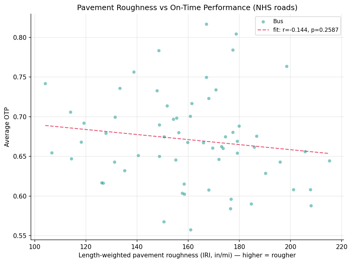
  • IRI vs OTP (bivariate): r = −0.144, p = 0.259 (n = 63 routes) -- not significant.
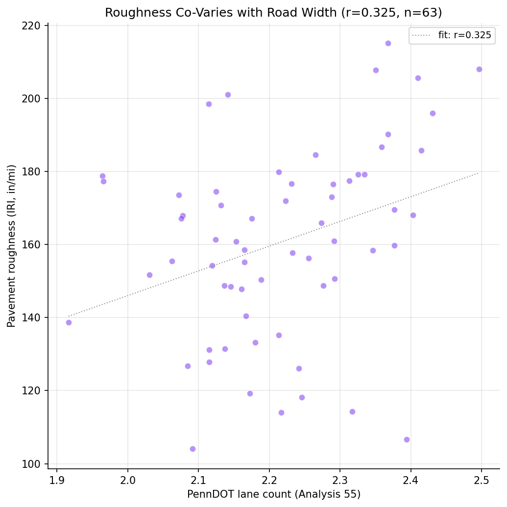
  • The confound is real: IRI vs lane count r = +0.325, p = 0.009. Rougher NHS pavement is on the wider arterials.
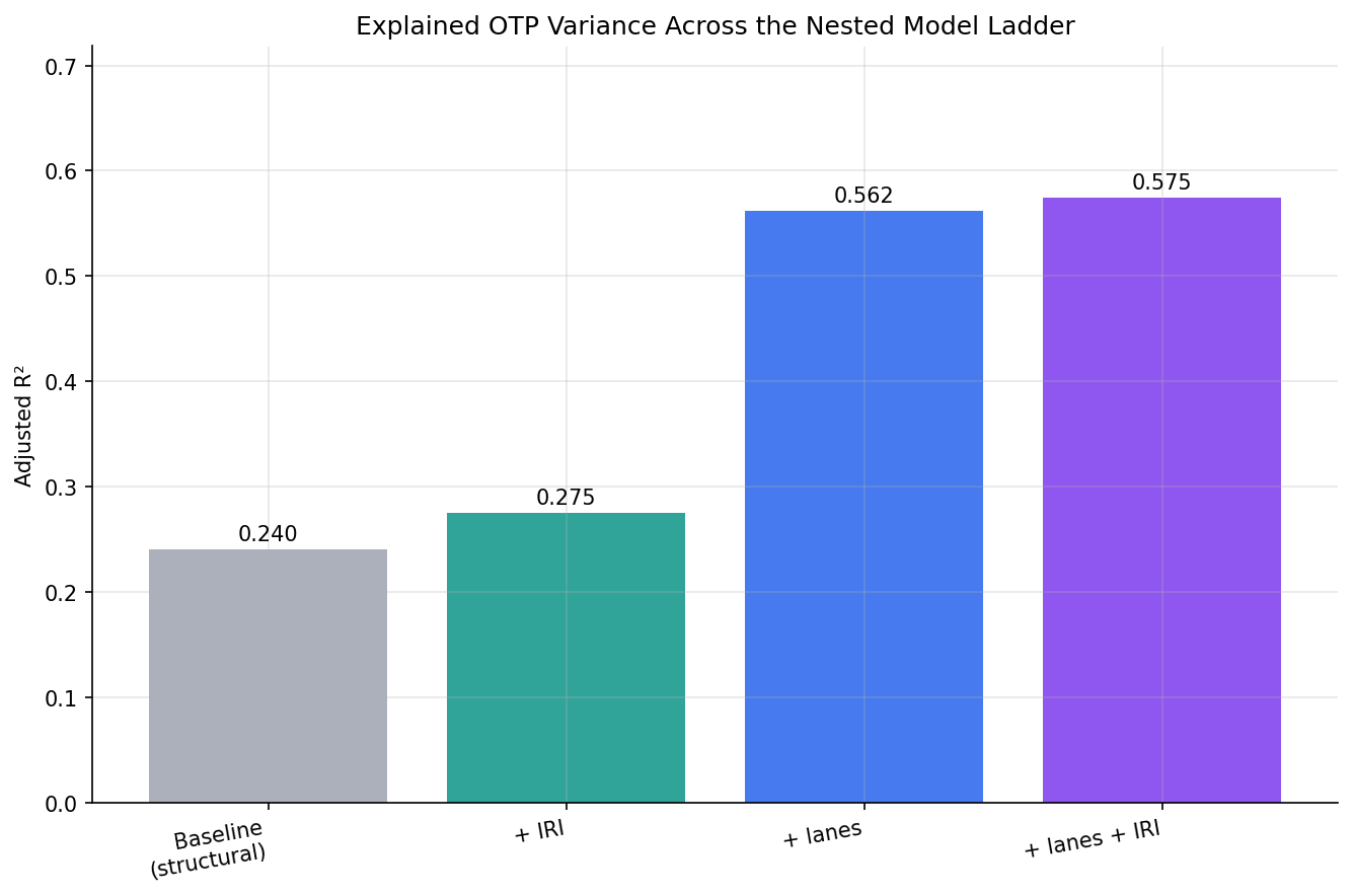
  • IRI over the structural baseline (no width control): F = 3.74, p = 0.058 -- marginal, adj R² 0.240 → 0.275.
  • IRI net of lane count (the decisive test): F = 2.68, p = 0.107 -- not significant. Adj R² 0.562 → 0.575 (+0.013).
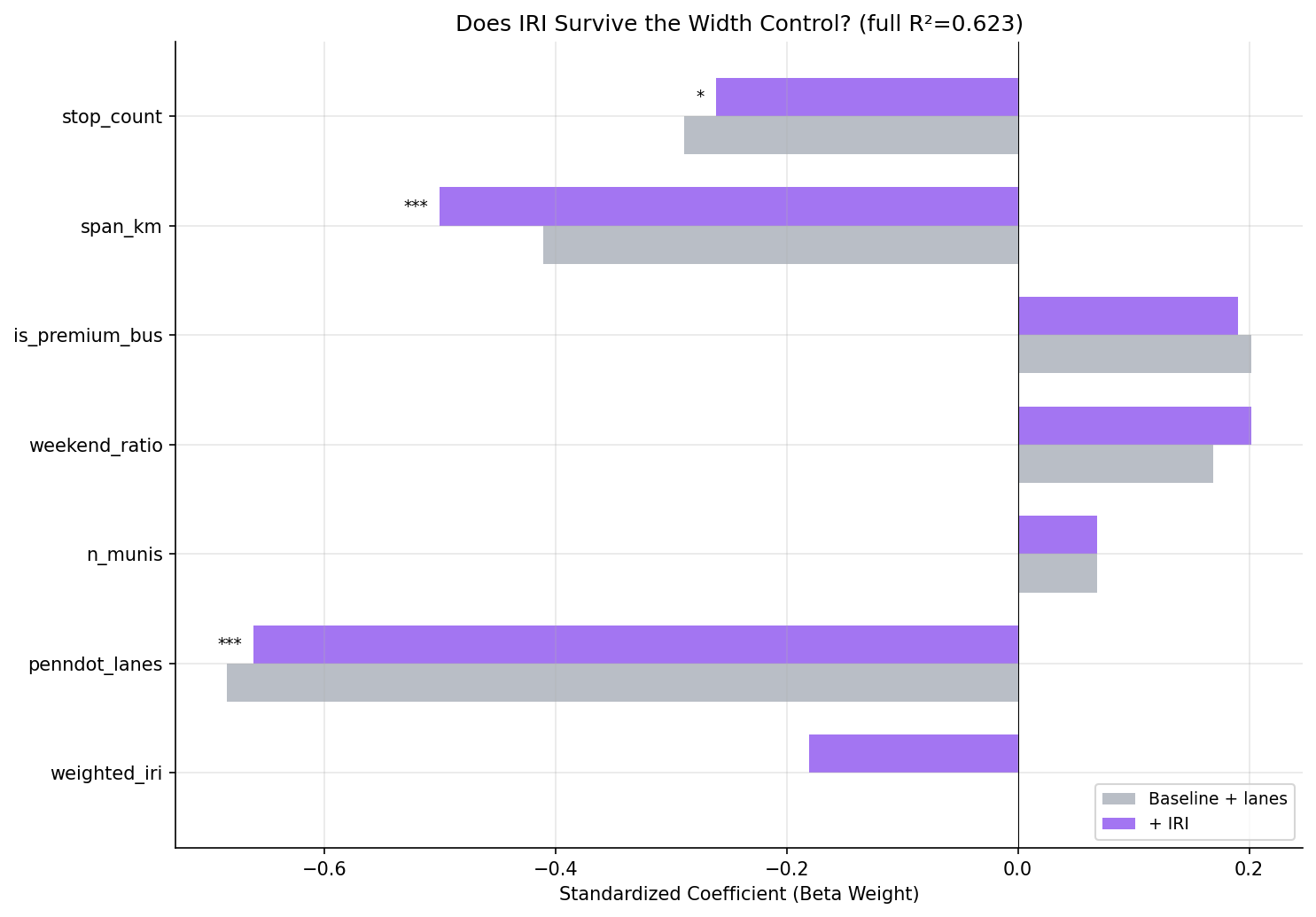
  • Lane count, by contrast, dominates: β = −0.68, p < 0.0001; adding it lifts adj R² 0.240 → 0.562 (F = 42.9).
  • No collinearity excuse: in the full model VIF = 1.78 for IRI and 1.57 for lane count (all predictors < 5). IRI had independent variance available and still added nothing.
  • Coverage: 63 of 92 routes clear NHS match_rate ≥ 0.3; median NHS coverage 52%. IRI range 104–215 in/mi (mean 161).

Observations

  • Pavement roughness does not survive the road-width control. The headline question was whether road quality explains OTP beyond road geometry. It does not. Lane count absorbs essentially all of the road-related signal; IRI's marginal contribution after controlling for width is statistically indistinguishable from zero.
  • The raw IRI hint is a confound, not a finding. Bivariately IRI is weakly negative (rougher → later) but not significant, and it co-varies with lane count (r = +0.33). This is exactly the trap flagged before the analysis: the roughest roads are busy arterials. Treating the raw correlation as a pavement effect would have been wrong.
  • poor_share runs the "wrong" way and is not robust. The share of a route on poor-rated pavement is weakly positively correlated with OTP (r = +0.29, p = 0.02) -- i.e., more poor pavement, slightly better on-time. This sign flip (opposite to the continuous IRI measure) is a hallmark of a confounded bivariate, not a real protective effect of bad roads; it is reported descriptively and excluded from the regression.
  • Rail dropped out of the sample, as expected. All 63 included routes are bus. The light-rail lines (BLUE, RED, SILVER) run on their own right-of-way, not NHS roads, so they fall below the coverage threshold -- a sanity check that the spatial match behaves.
  • This complements, not contradicts, Analyses 55/56. Those found road width matters; this finds that, given width, surface condition does not. Together they sharpen the mechanism: the road-type effect operates through arterial geometry and the traffic/stop environment it implies, not through ride quality.

Caveats

  • Area-level (ecological) association. This is a route-level relationship between the roads a route runs along and its aggregate OTP, not an individual-trip causal claim.
  • NHS-only coverage. The pavement layer covers the National Highway System (interstates and principal arterials) only, so each route's IRI characterizes its major-arterial running, not its local-street segments. 29 routes with < 30% NHS coverage were excluded; the included routes have median 52% coverage.
  • A null is not proof of no effect. With n = 63 the analysis is powered to detect a moderate independent IRI effect; a small one could be missed. The point estimate is small and the same sign as the (confounded) bivariate, so a large hidden effect is unlikely, but this rules out a strong pavement→OTP relationship, not a tiny one.
  • IRI measures roughness, not all pavement distress. Potholes, patching, and work-zone repaving -- which could plausibly affect buses more acutely than average roughness -- are not captured by a length-weighted IRI mean.
  • Static snapshot. Pavement condition and OTP are each aggregated over time, not matched month-to-month, so this cannot detect whether a repaving event changed a route's reliability.

Validation

Data inputs

  1. Data source verified. route_road_pavement columns checked against prt_otp_analysis.common.schemas.ROUTE_ROAD_PAVEMENT and validated at load (validate(..., subset=True)). Pavement fields (ROUGH_INDX, OVERALL_PV, IRI_RATING) confirmed against the live SPC service before building (see data/spc-pavement/SOURCE.md).
  2. Geographic/temporal scope matches. OTP averaged over routes with 12+ months; IRI matched to the same GTFS route shapes used throughout the project (30 m buffer, identical KDTree machinery as Analyses 27/55/56). The lane-count control comes from route_road_class (Analysis 55) on the same routes; all 63 pavement-matched routes also clear the lane match threshold, so Q1 and Q2 use one identical sample.
  3. Null/missing handling. IRI is filtered to > 0 at query time; OPI 0 treated as missing. Routes with NHS match_rate < 0.3 excluded, not imputed.

Results plausibility

  1. Aggregates sanity-checked. Mean IRI 161 in/mi (range 104–215) is consistent with FAIR-to-POOR urban arterial pavement; the roughest routes (71A–D, 88, 61A) are known busy corridors. Values are in the expected band for NHS roads.
  2. Surprising results investigated. The result is not surprising and is the honest outcome: the raw IRI hint was anticipated to be a road-width confound, and it is. The poor_share sign flip was investigated and attributed to confounding, not reported as a protective effect.
  3. Direction of effects checked. Lane count reproduces the Analysis 55/56 negative sign and dominates; stop count and span negative; n_munis positive -- all consistent with prior structural models.

Statistical diagnostics

  1. Multicollinearity checked. VIF reported for all predictors in the full model; max is is_premium_bus at 3.34. IRI = 1.78, lane count = 1.57. No predictor exceeds 5, so the null IRI result is not a collinearity artifact.
  2. Small-sample routes flagged. Minimum 12 months of OTP and NHS match_rate ≥ 0.3 enforced; n = 63 routes (all bus). Constant dummy columns (is_rail, with no rail in the sample) are dropped before fitting so the design matrix stays well-conditioned.
  3. Ecological framing. Results described as route/area-level associations throughout; no individual-trip causal claim is made.

Output
Methods

Methods: Pavement Condition and OTP

Question

Analyses 55 and 56 established that road width (lane count) is a robust correlate of on-time performance: buses on wider, multi-lane roads run late more often. But both measured road geometry. They never tested road quality. SPC's National Highway System pavement-condition layer adds one attribute neither dataset has: pavement roughness, the International Roughness Index (IRI). This analysis asks two questions:

  1. Does pavement roughness correlate with OTP at all? Rougher pavement plausibly forces slower, more variable bus speeds.
  2. Does roughness add explanatory power net of road width? This is the decisive question. The roughest roads are busy urban arterials -- which are also the wide, multi-lane roads we already know run late. So a raw IRI->OTP correlation is almost certainly confounded with lane count. The honest test is whether IRI survives once road width is controlled. A null here is itself a clean finding: it would mean the road-type signal is about geometry (how a road channels traffic and stops), not the physical condition of the surface.

This is deliberately framed as a confound-aware test, not a hunt for a positive result.

Approach

  • Build route_road_pavement (pipeline step 14): for each route, the length-weighted mean IRI of NHS pavement segments within 30 m of its GTFS shape, plus the length-weighted overall pavement index (OPI) and the share of length rated POOR. Match rate records the within-buffer (≈ on-NHS) fraction of the route.
  • Include routes with 12+ months of OTP and route_road_pavement.match_rate >= 0.3.
  • Bivariate: correlate IRI with OTP. Also correlate IRI with the PennDOT lane count (Analysis 55's route_road_class.weighted_lanes) to quantify the confound directly.
  • Regression (the core): replicate the Analysis 18/55 six-feature structural OLS baseline on the pavement-matched sample, then build a nested ladder:
    • Model A: structural baseline (6 features).
    • Model B: baseline + IRI (does roughness matter beyond structure?).
    • Model C: baseline + lane count (the road-width control).
    • Model D: baseline + lane count + IRI (does IRI survive controlling for width?). Test each addition with a nested F-test; compute VIF for the full model and flag any predictor with VIF > 5 (IRI and lane count are expected to be correlated).
  • Report OPI and poor-share descriptively (Pearson r with OTP).
  • Repeat the baseline-vs-IRI comparison on the bus-only subset.

All regression helpers (compute_span, fit_ols, compute_vif, f_test_nested) are replicated locally so the analysis does not import from Analysis 18/55/56 (analyses must be independent).

Data

Name Description Source
otp_monthly route_id, month, otp (averaged to route level, 12+ months required) prt.db table
route_road_pavement route_id, weighted_iri, weighted_opi, poor_share, match_rate (built by road_overlay_pavement.py, pipeline step 14) prt.db table
route_road_class route_id, weighted_lanes (PennDOT, the road-width control) prt.db table
route_stops stop counts, trip frequencies prt.db table
stops lat, lon for geographic span; muni for municipality count prt.db table
routes route_id, mode for subtype classification prt.db table

Inclusion: routes with 12+ months of OTP and route_road_pavement.match_rate >= 0.3. IRI is length-weighted over the NHS pavement segments within 30 m of the route's GTFS shape. The layer is NHS-only (interstates and principal arterials), so each route's IRI characterizes only its major-arterial running; the match rate quantifies the covered share. The lane-count control models are fit on the subset of routes that also clear route_road_class.match_rate >= 0.3.

Output

  • output/model_comparison.csv -- regression results (baseline, +IRI, +lanes, +lanes+IRI, bus subset)
  • output/vif_table.csv -- VIF values for the full model
  • output/route_pavement_summary.csv -- per-route IRI, OPI, poor-share, lane count, OTP
  • output/iri_vs_otp.png -- bivariate scatter of IRI vs OTP
  • output/iri_vs_lanes.png -- IRI vs lane count, showing the confound
  • output/r2_progression.png -- adjusted R² across the nested model ladder
  • output/coefficient_comparison.png -- beta weights, baseline vs full model

Source Code

"""Analysis 57: Test whether pavement roughness (IRI) predicts OTP, and whether
that signal survives controlling for road width (lane count from Analysis 55)."""

import math

import numpy as np
import polars as pl
from scipy import stats

from prt_otp_analysis.common import (
    analysis_dir,
    classify_bus_route,
    correlate,
    phase,
    query_to_polars,
    run_analysis,
    save_chart,
    save_csv,
    setup_plotting,
)
from prt_otp_analysis.common.schemas import ROUTE_ROAD_PAVEMENT, validate

OUT = analysis_dir(__file__)

MIN_MONTHS = 12
MIN_MATCH_RATE = 0.3


# ---------------------------------------------------------------------------
# Helpers (replicated from Analysis 18/55/56 to keep analyses independent)
# ---------------------------------------------------------------------------

def haversine_km(lat1: float, lon1: float, lat2: float, lon2: float) -> float:
    """Return the great-circle distance in km between two lat/lon points."""
    R = 6371.0
    dlat = math.radians(lat2 - lat1)
    dlon = math.radians(lon2 - lon1)
    a = (math.sin(dlat / 2) ** 2
         + math.cos(math.radians(lat1)) * math.cos(math.radians(lat2))
         * math.sin(dlon / 2) ** 2)
    return R * 2 * math.atan2(math.sqrt(a), math.sqrt(1 - a))


def compute_span(lats: list[float], lons: list[float]) -> float:
    """Return the max pairwise haversine distance (km) among a set of points."""
    max_dist = 0.0
    n = len(lats)
    for i in range(n):
        for j in range(i + 1, n):
            d = haversine_km(lats[i], lons[i], lats[j], lons[j])
            if d > max_dist:
                max_dist = d
    return max_dist


def compute_vif(X_raw: np.ndarray, feature_names: list[str]) -> dict[str, float]:
    """Compute Variance Inflation Factor for each predictor."""
    n, k = X_raw.shape
    vifs = {}
    for j in range(k):
        y_j = X_raw[:, j]
        X_other = np.delete(X_raw, j, axis=1)
        X_other = np.column_stack([np.ones(n), X_other])
        beta, _, _, _ = np.linalg.lstsq(X_other, y_j, rcond=None)
        y_hat = X_other @ beta
        ss_res = np.sum((y_j - y_hat) ** 2)
        ss_tot = np.sum((y_j - np.mean(y_j)) ** 2)
        r2_j = 1 - ss_res / ss_tot if ss_tot > 0 else 0.0
        vifs[feature_names[j]] = 1.0 / (1.0 - r2_j) if r2_j < 1.0 else float("inf")
    return vifs


def fit_ols(y: np.ndarray, X_raw: np.ndarray, feature_names: list[str]) -> dict:
    """Fit OLS regression and return results dict."""
    n, k = X_raw.shape
    X = np.column_stack([np.ones(n), X_raw])

    beta, _, _, _ = np.linalg.lstsq(X, y, rcond=None)
    y_hat = X @ beta
    residuals = y - y_hat

    ss_res = np.sum(residuals ** 2)
    ss_tot = np.sum((y - np.mean(y)) ** 2)
    r_squared = 1 - ss_res / ss_tot
    adj_r_squared = 1 - (1 - r_squared) * (n - 1) / (n - k - 1)
    mse = ss_res / (n - k - 1)

    XtX_inv = np.linalg.pinv(X.T @ X)
    se = np.sqrt(np.diag(XtX_inv) * mse)
    t_vals = beta / se
    p_vals = [2 * (1 - stats.t.cdf(abs(t), df=n - k - 1)) for t in t_vals]

    x_stds = np.std(X_raw, axis=0, ddof=1)
    y_std = np.std(y, ddof=1)
    beta_weights = beta[1:] * x_stds / y_std

    return {
        "r_squared": r_squared,
        "adj_r_squared": adj_r_squared,
        "ss_res": ss_res,
        "n": n,
        "k": k,
        "features": ["intercept"] + feature_names,
        "coefficients": beta.tolist(),
        "std_errors": se.tolist(),
        "t_values": t_vals.tolist(),
        "p_values": p_vals,
        "beta_weights": [None] + beta_weights.tolist(),
        "y_hat": y_hat,
        "residuals": residuals,
    }


def f_test_nested(base: dict, full: dict) -> tuple[float, float]:
    """F-test comparing nested models. Returns (F_stat, p_value)."""
    k_diff = full["k"] - base["k"]
    n = full["n"]
    f_stat = ((base["ss_res"] - full["ss_res"]) / k_diff) / (full["ss_res"] / (n - full["k"] - 1))
    f_p = 1 - stats.f.cdf(f_stat, k_diff, n - full["k"] - 1)
    return f_stat, f_p


def print_model(results: dict, label: str) -> None:
    """Print formatted model results."""
    print(f"\n  {label}:")
    print(f"  R2 = {results['r_squared']:.4f}, Adj R2 = {results['adj_r_squared']:.4f}, "
          f"n = {results['n']}, k = {results['k']}")
    print(f"  {'Feature':<20s} {'Coeff':>10s} {'Std Err':>10s} {'p-value':>10s} {'Beta':>10s}")
    print(f"  {'-'*60}")
    for i, feat in enumerate(results["features"]):
        coeff = results["coefficients"][i]
        se = results["std_errors"][i]
        p = results["p_values"][i]
        beta = results["beta_weights"][i]
        beta_str = f"{beta:>10.4f}" if beta is not None else f"{'--':>10s}"
        sig = "***" if p < 0.001 else "**" if p < 0.01 else "*" if p < 0.05 else ""
        print(f"  {feat:<20s} {coeff:>10.6f} {se:>10.6f} {p:>10.4f} {beta_str} {sig}")


def vary(df: pl.DataFrame, features: list[str]) -> list[str]:
    """Keep only features with more than one unique value in this sample.

    Dummies like is_rail can be constant on the NHS-only subset (rail routes run
    on their own right-of-way and drop out), which would make them collinear with
    the intercept; drop them so the design matrix stays well-conditioned.
    """
    return [f for f in features if df[f].n_unique() > 1]


# ---------------------------------------------------------------------------
# Data loading
# ---------------------------------------------------------------------------

def load_features() -> pl.DataFrame:
    """Assemble structural features + pavement (IRI) + PennDOT lane count."""
    avg_otp_df = query_to_polars(f"""
        SELECT o.route_id, r.route_name, r.mode,
               AVG(o.otp) AS avg_otp, COUNT(*) AS months
        FROM otp_monthly o
        JOIN routes r ON o.route_id = r.route_id
        GROUP BY o.route_id
        HAVING COUNT(*) >= {MIN_MONTHS}
    """)

    stop_counts_df = query_to_polars("""
        SELECT route_id, COUNT(DISTINCT stop_id) AS stop_count
        FROM route_stops GROUP BY route_id
    """)
    trips_df = query_to_polars("""
        SELECT route_id,
               MAX(trips_wd) AS max_wd,
               MAX(trips_sa) AS max_sa,
               MAX(trips_su) AS max_su
        FROM route_stops GROUP BY route_id
    """)
    munis_df = query_to_polars("""
        SELECT rs.route_id, COUNT(DISTINCT s.muni) AS n_munis
        FROM route_stops rs
        JOIN stops s ON rs.stop_id = s.stop_id
        WHERE s.muni IS NOT NULL AND s.muni != '0'
        GROUP BY rs.route_id
    """)
    stops_by_route_df = query_to_polars("""
        SELECT rs.route_id, s.lat, s.lon
        FROM route_stops rs
        JOIN stops s ON rs.stop_id = s.stop_id
        WHERE s.lat IS NOT NULL AND s.lon IS NOT NULL
    """)
    spans = []
    for route_id in stops_by_route_df["route_id"].unique().sort().to_list():
        subset = stops_by_route_df.filter(pl.col("route_id") == route_id)
        span_km = compute_span(subset["lat"].to_list(), subset["lon"].to_list())
        spans.append({"route_id": route_id, "span_km": span_km})
    span_df = pl.DataFrame(spans)

    pavement_df = query_to_polars("""
        SELECT route_id, weighted_iri, weighted_opi, poor_share,
               match_rate, n_segments, total_length_ft
        FROM route_road_pavement
    """)
    validate(pavement_df, ROUTE_ROAD_PAVEMENT, subset=True)

    # PennDOT lane count: the road-width control (Analysis 55).
    penndot_df = query_to_polars("""
        SELECT route_id, weighted_lanes AS penndot_lanes,
               match_rate AS penndot_match_rate
        FROM route_road_class
    """)

    df = avg_otp_df
    df = df.join(stop_counts_df, on="route_id", how="left")
    df = df.join(trips_df, on="route_id", how="left")
    df = df.join(munis_df, on="route_id", how="left")
    df = df.join(span_df, on="route_id", how="left")
    df = df.join(pavement_df, on="route_id", how="inner")
    df = df.join(penndot_df, on="route_id", how="left")

    df = df.with_columns(
        pl.when(pl.col("max_wd") > 0)
        .then((pl.col("max_sa") + pl.col("max_su")) / (2.0 * pl.col("max_wd")))
        .otherwise(0.0)
        .alias("weekend_ratio"),
    )
    df = df.with_columns(
        pl.when(pl.col("mode") == "RAIL").then(1.0).otherwise(0.0).alias("is_rail"),
    )
    df = df.with_columns(
        pl.when(pl.col("mode") == "BUS")
        .then(pl.col("route_id").map_elements(classify_bus_route, return_dtype=pl.Utf8))
        .otherwise(pl.lit("non_bus"))
        .alias("bus_subtype"),
    )
    df = df.with_columns(
        pl.when(pl.col("bus_subtype").is_in(["busway", "flyer", "express", "limited"]))
        .then(1.0)
        .otherwise(0.0)
        .alias("is_premium_bus"),
    )

    df = df.drop_nulls(subset=["stop_count", "span_km", "weekend_ratio", "n_munis", "weighted_iri"])
    return df


# ---------------------------------------------------------------------------
# Charts
# ---------------------------------------------------------------------------

def make_iri_scatter(df: pl.DataFrame) -> None:
    """Bivariate scatter: pavement roughness (IRI) vs OTP."""
    plt = setup_plotting()
    fig, ax = plt.subplots(figsize=(8, 6))

    iri = df["weighted_iri"].to_numpy()
    otp = df["avg_otp"].to_numpy()
    modes = df["mode"].to_list()
    bus_mask = np.array([m == "BUS" for m in modes])
    rail_mask = ~bus_mask

    ax.scatter(iri[bus_mask], otp[bus_mask], alpha=0.5, s=30, color="#0d9488",
               edgecolors="white", linewidth=0.5, label="Bus", zorder=2)
    if np.any(rail_mask):
        ax.scatter(iri[rail_mask], otp[rail_mask], alpha=0.7, s=50, color="#dc2626",
                   marker="D", edgecolors="white", linewidth=0.5, label="Rail", zorder=3)

    slope, intercept, r, p, _ = stats.linregress(iri, otp)
    x_line = np.array([iri.min(), iri.max()])
    ax.plot(x_line, slope * x_line + intercept, color="#e11d48", linewidth=1.5,
            linestyle="--", alpha=0.7, label=f"fit: r={r:.3f}, p={p:.4f}")

    ax.set_xlabel("Length-weighted pavement roughness (IRI, in/mi) — higher = rougher")
    ax.set_ylabel("Average OTP")
    ax.set_title("Pavement Roughness vs On-Time Performance (NHS roads)")
    ax.legend(fontsize=9)
    save_chart(fig, OUT / "iri_vs_otp.png")


def make_iri_vs_lanes(df: pl.DataFrame) -> None:
    """Scatter of IRI vs PennDOT lane count, showing the road-width confound."""
    plt = setup_plotting()
    fig, ax = plt.subplots(figsize=(7, 7))

    sub = df.drop_nulls(subset=["penndot_lanes"]).filter(
        pl.col("penndot_match_rate") >= MIN_MATCH_RATE
    )
    iri = sub["weighted_iri"].to_numpy()
    lanes = sub["penndot_lanes"].to_numpy()

    ax.scatter(lanes, iri, alpha=0.55, s=35, color="#7c3aed",
               edgecolors="white", linewidth=0.5, zorder=2)
    slope, intercept, r, p, _ = stats.linregress(lanes, iri)
    x_line = np.array([lanes.min(), lanes.max()])
    ax.plot(x_line, slope * x_line + intercept, color="gray", linewidth=1.0,
            linestyle=":", alpha=0.8, label=f"fit: r={r:.3f}")
    ax.set_xlabel("PennDOT lane count (Analysis 55)")
    ax.set_ylabel("Pavement roughness (IRI, in/mi)")
    ax.set_title(f"Roughness Co-Varies with Road Width (r={r:.3f}, n={len(sub)})")
    ax.legend(fontsize=9)
    save_chart(fig, OUT / "iri_vs_lanes.png")


def make_r2_progression(model_specs: list[tuple[str, dict]]) -> None:
    """Bar chart of adjusted R^2 across the nested ladder (same sample)."""
    plt = setup_plotting()
    fig, ax = plt.subplots(figsize=(9, 6))

    labels = [label for label, _ in model_specs]
    adj_r2 = [m["adj_r_squared"] for _, m in model_specs]
    colors = ["#9ca3af", "#0d9488", "#2563eb", "#7c3aed"][: len(labels)]

    bars = ax.bar(labels, adj_r2, color=colors, alpha=0.85)
    for bar, val in zip(bars, adj_r2):
        ax.text(bar.get_x() + bar.get_width() / 2, val + 0.005, f"{val:.3f}",
                ha="center", va="bottom", fontsize=10)

    ax.set_ylabel("Adjusted R²")
    ax.set_title("Explained OTP Variance Across the Nested Model Ladder")
    ax.set_ylim(0, max(adj_r2) * 1.25)
    plt.xticks(rotation=10, ha="right")
    save_chart(fig, OUT / "r2_progression.png")


def make_coefficient_chart(base: dict, full: dict) -> None:
    """Compare standardized coefficients between baseline and full (+lanes+IRI) model."""
    plt = setup_plotting()
    fig, ax = plt.subplots(figsize=(10, 7))

    full_feats = full["features"][1:]
    base_betas = {f: b for f, b in zip(base["features"][1:], base["beta_weights"][1:])}
    full_betas = {f: b for f, b in zip(full_feats, full["beta_weights"][1:])}
    full_pvals = {f: p for f, p in zip(full_feats, full["p_values"][1:])}

    y_pos = np.arange(len(full_feats))
    width = 0.35
    base_vals = [base_betas.get(f, 0.0) for f in full_feats]
    full_vals = [full_betas[f] for f in full_feats]

    ax.barh(y_pos + width / 2, base_vals, width, label="Baseline + lanes",
            color="#9ca3af", alpha=0.7)
    ax.barh(y_pos - width / 2, full_vals, width, label="+ IRI",
            color="#7c3aed", alpha=0.7)

    for i, f in enumerate(full_feats):
        p = full_pvals[f]
        marker = "***" if p < 0.001 else "**" if p < 0.01 else "*" if p < 0.05 else ""
        val = full_vals[i]
        ax.text(val + 0.01 if val >= 0 else val - 0.01, i - width / 2, marker,
                ha="left" if val >= 0 else "right", va="center", fontsize=9)

    ax.set_yticks(y_pos)
    ax.set_yticklabels(full_feats)
    ax.axvline(0, color="black", linewidth=0.5)
    ax.set_xlabel("Standardized Coefficient (Beta Weight)")
    ax.set_title(f"Does IRI Survive the Width Control? "
                 f"(full R²={full['r_squared']:.3f})")
    ax.legend(loc="lower right", fontsize=9)
    ax.invert_yaxis()
    save_chart(fig, OUT / "coefficient_comparison.png")


# ---------------------------------------------------------------------------
# Main
# ---------------------------------------------------------------------------

@run_analysis(57, "Pavement Condition and OTP")
def main() -> None:
    """Entry point: test IRI->OTP and whether it survives the road-width control."""

    with phase("Loading and assembling features"):
        df_all = load_features()
        df = df_all.filter(pl.col("match_rate") >= MIN_MATCH_RATE)
        excluded = df_all.filter(pl.col("match_rate") < MIN_MATCH_RATE)
        n_rail = len(df.filter(pl.col("is_rail") == 1.0))
        n_bus = len(df.filter(pl.col("mode") == "BUS"))
        print(f"  {len(df)} routes after match_rate >= {MIN_MATCH_RATE} filter "
              f"({n_bus} BUS, {n_rail} RAIL)")
        if len(excluded) > 0:
            print(f"  Excluded ({len(excluded)}, low NHS coverage): "
                  + ", ".join(excluded.sort("match_rate")["route_id"].to_list()))
        print(f"\n  IRI range: {df['weighted_iri'].min():.0f} -- "
              f"{df['weighted_iri'].max():.0f} (mean {df['weighted_iri'].mean():.0f} in/mi)")
        print(f"  Median NHS match rate: {df['match_rate'].median():.1%}")

    y = df["avg_otp"].to_numpy()

    # --- Bivariate: IRI vs OTP, and the confound IRI vs lane count ---
    with phase("Bivariate associations"):
        c_otp = correlate(df, "weighted_iri", "avg_otp")
        print(f"  IRI vs OTP:           r = {c_otp['pearson_r']:+.3f}, "
              f"p = {c_otp['pearson_p']:.4f} (n={len(df)})")
        for feat in ["weighted_opi", "poor_share"]:
            sub = df.drop_nulls(subset=[feat])
            c = correlate(sub, feat, "avg_otp")
            sig = "*" if c["pearson_p"] < 0.05 else ""
            print(f"  {feat:<20s} r = {c['pearson_r']:+.3f}, "
                  f"p = {c['pearson_p']:.4f} (n={len(sub)}) {sig}")
        width_df = df.drop_nulls(subset=["penndot_lanes"]).filter(
            pl.col("penndot_match_rate") >= MIN_MATCH_RATE
        )
        c_conf = correlate(width_df, "weighted_iri", "penndot_lanes")
        print(f"\n  CONFOUND -- IRI vs lane count: r = {c_conf['pearson_r']:+.3f}, "
              f"p = {c_conf['pearson_p']:.4f} (n={len(width_df)})")
        print("  (Rougher roads tend to be the wider arterials we already know run late.)")

    cand_base = ["stop_count", "span_km", "is_rail", "is_premium_bus",
                 "weekend_ratio", "n_munis"]

    # --- Q1: does IRI matter beyond structure? (pavement sample) ---
    base_features = vary(df, cand_base)
    X_base = np.column_stack([df[f].to_numpy().astype(float) for f in base_features])
    X_base_iri = np.column_stack([df[f].to_numpy().astype(float)
                                  for f in base_features + ["weighted_iri"]])
    with phase("Q1: structural baseline vs + IRI (pavement sample)"):
        base = fit_ols(y, X_base, base_features)
        base_iri = fit_ols(y, X_base_iri, base_features + ["weighted_iri"])
        print_model(base, f"Structural baseline ({len(base_features)} features)")
        print_model(base_iri, "Baseline + IRI")
        f1, p1 = f_test_nested(base, base_iri)
        print(f"\n  F-test for IRI (no width control): F = {f1:.3f}, p = {p1:.4f}")
        print(f"  Adj R2: {base['adj_r_squared']:.4f} -> {base_iri['adj_r_squared']:.4f} "
              f"(+{base_iri['adj_r_squared'] - base['adj_r_squared']:.4f})")

    # --- Q2: does IRI survive the road-width control? (width sample) ---
    with phase(f"Q2: IRI net of lane count (width sample, n={len(width_df)})"):
        yw = width_df["avg_otp"].to_numpy()
        wbase_feats = vary(width_df, cand_base)
        w_lane_feats = wbase_feats + ["penndot_lanes"]
        w_iri_feats = wbase_feats + ["weighted_iri"]
        w_full_feats = wbase_feats + ["penndot_lanes", "weighted_iri"]

        Xw_base = np.column_stack([width_df[f].to_numpy().astype(float) for f in wbase_feats])
        Xw_lane = np.column_stack([width_df[f].to_numpy().astype(float) for f in w_lane_feats])
        Xw_iri = np.column_stack([width_df[f].to_numpy().astype(float) for f in w_iri_feats])
        Xw_full = np.column_stack([width_df[f].to_numpy().astype(float) for f in w_full_feats])

        wbase = fit_ols(yw, Xw_base, wbase_feats)
        w_lane = fit_ols(yw, Xw_lane, w_lane_feats)
        w_iri = fit_ols(yw, Xw_iri, w_iri_feats)
        w_full = fit_ols(yw, Xw_full, w_full_feats)

        print_model(w_lane, "Baseline + lane count")
        print_model(w_full, "Baseline + lane count + IRI")
        f_lane, p_lane = f_test_nested(wbase, w_lane)
        f_iri_only, p_iri_only = f_test_nested(wbase, w_iri)
        f_net, p_net = f_test_nested(w_lane, w_full)
        print(f"\n  Lane count over baseline:      F = {f_lane:.3f}, p = {p_lane:.4f} "
              f"(Adj R2 {wbase['adj_r_squared']:.4f} -> {w_lane['adj_r_squared']:.4f})")
        print(f"  IRI alone over baseline:       F = {f_iri_only:.3f}, p = {p_iri_only:.4f} "
              f"(Adj R2 {wbase['adj_r_squared']:.4f} -> {w_iri['adj_r_squared']:.4f})")
        print(f"  *** IRI NET OF LANE COUNT:     F = {f_net:.3f}, p = {p_net:.4f} "
              f"(Adj R2 {w_lane['adj_r_squared']:.4f} -> {w_full['adj_r_squared']:.4f}) ***")
        if p_net < 0.05:
            print("  => IRI SURVIVES the road-width control: pavement quality adds signal.")
        else:
            print("  => IRI does NOT survive: the road signal is geometry, not surface condition.")

    # --- VIF on the full model ---
    with phase("VIF (full model: baseline + lanes + IRI)"):
        vifs = compute_vif(Xw_full, w_full_feats)
        for feat, vif in vifs.items():
            flag = " ** HIGH" if vif > 5 else ""
            print(f"  {feat:<20s} VIF = {vif:.2f}{flag}")

    # --- Bus-only subgroup (Q1 on buses) ---
    bus_df = df.filter(pl.col("mode") == "BUS")
    with phase(f"Bus-only: baseline vs + IRI ({len(bus_df)} routes)"):
        y_bus = bus_df["avg_otp"].to_numpy()
        bus_base_feats = vary(bus_df, ["stop_count", "span_km", "is_premium_bus",
                                       "weekend_ratio", "n_munis"])
        bus_full_feats = bus_base_feats + ["weighted_iri"]
        X_bus_base = np.column_stack([bus_df[f].to_numpy().astype(float) for f in bus_base_feats])
        X_bus_full = np.column_stack([bus_df[f].to_numpy().astype(float) for f in bus_full_feats])
        bus_base = fit_ols(y_bus, X_bus_base, bus_base_feats)
        bus_full = fit_ols(y_bus, X_bus_full, bus_full_feats)
        f_b, fp_b = f_test_nested(bus_base, bus_full)
        print(f"  Bus-only F-test for IRI: F = {f_b:.3f}, p = {fp_b:.4f}")
        print(f"  Adj R2: {bus_base['adj_r_squared']:.4f} -> {bus_full['adj_r_squared']:.4f}")

    with phase("Saving CSVs"):
        rows = []
        models = [
            (base, "base"),
            (base_iri, "base_plus_iri"),
            (w_lane, "width_base_plus_lanes"),
            (w_full, "width_base_plus_lanes_iri"),
            (bus_base, "bus_base"),
            (bus_full, "bus_plus_iri"),
        ]
        for model, label in models:
            for i, feat in enumerate(model["features"]):
                bw = model["beta_weights"][i]
                rows.append({
                    "model": label,
                    "feature": feat,
                    "coefficient": model["coefficients"][i],
                    "std_error": model["std_errors"][i],
                    "p_value": model["p_values"][i],
                    "beta_weight": bw if bw is not None else float("nan"),
                    "r_squared": model["r_squared"],
                    "adj_r_squared": model["adj_r_squared"],
                    "n": model["n"],
                })
        save_csv(pl.DataFrame(rows), OUT / "model_comparison.csv")

        vif_df = pl.DataFrame([{"feature": f, "vif": v} for f, v in vifs.items()])
        save_csv(vif_df, OUT / "vif_table.csv")

        summary_df = df.select([
            "route_id", "route_name", "mode", "avg_otp",
            "weighted_iri", "weighted_opi", "poor_share", "penndot_lanes",
            "match_rate", "penndot_match_rate", "n_segments", "stop_count", "span_km",
        ]).sort("weighted_iri", descending=True)
        save_csv(summary_df, OUT / "route_pavement_summary.csv")

    with phase("Generating charts"):
        make_iri_scatter(df)
        make_iri_vs_lanes(df)
        make_r2_progression([
            ("Baseline\n(structural)", wbase),
            ("+ IRI", w_iri),
            ("+ lanes", w_lane),
            ("+ lanes + IRI", w_full),
        ])
        make_coefficient_chart(w_lane, w_full)


if __name__ == "__main__":
    main()

Sources

NameTypeWhy It MattersOwnerFreshnessCaveat
otp_monthly table Primary analytical table used in this page's computations. Produced by Data Ingestion. Updated when the producing pipeline step is rerun. Coverage depends on upstream source availability and ETL assumptions.
Upstream sources (5)
  • file data/routes_by_month.csv — Monthly route OTP source table in wide format.
  • file data/PRT_Current_Routes_Full_System_de0e48fcbed24ebc8b0d933e47b56682.csv — Current route metadata and mode classifications.
  • file data/Transit_stops_(current)_by_route_e040ee029227468ebf9d217402a82fa9.csv — Current stop-to-route coverage and trip counts.
  • file data/PRT_Stop_Reference_Lookup_Table.csv — Historical stop reference file with geography attributes.
  • file data/average-ridership/12bb84ed-397e-435c-8d1b-8ce543108698.csv — Average ridership by route and month.
route_road_pavement table Primary analytical table used in this page's computations. Produced by NHS Pavement-Condition Overlay ETL. Updated when the producing pipeline step is rerun. Coverage depends on upstream source availability and ETL assumptions.
Upstream sources (4)
  • file data/spc-pavement/pavement_raw.geojson — Cached SPC NHS pavement-condition GeoJSON (ROUGH_INDX/IRI, OVERALL_PV, IRI_RATING, geometry) in WGS84.
  • file data/GTFS/shapes.txt — GTFS route shape geometry points.
  • file data/GTFS/trips.txt — GTFS shape-to-route mapping.
  • api SPC NHS Pavement Condition (PM2_Roadways, ArcGIS) — Southwestern Pennsylvania Commission feature service of NHS pavement condition (IRI roughness, overall pavement index, IRI rating) derived from PennDOT roadway-management data.
route_road_class table Primary analytical table used in this page's computations. Produced by Road Classification Overlay ETL. Updated when the producing pipeline step is rerun. Coverage depends on upstream source availability and ETL assumptions.
Upstream sources (6)
  • file data/penndot-roadclass/roadwaysegments.json — Cached PennDOT ArcGIS roadwaysegments response (lane count, median type, geometry) for Allegheny County.
  • file data/penndot-roadclass/roadwayadmin.json — Cached PennDOT ArcGIS roadwayadmin response (functional class, posted speed) for Allegheny County.
  • file data/GTFS/shapes.txt — GTFS route shape geometry points.
  • file data/GTFS/trips.txt — GTFS shape-to-route mapping.
  • api PennDOT ArcGIS Roadway Segments Layer (RMSSEG) — Public state-roadway segment attributes including lane count and median type.
  • api PennDOT ArcGIS Roadway Admin Layer — Public roadway administrative attributes including FHWA functional class and posted speed limit.
route_stops table Primary analytical table used in this page's computations. Produced by Data Ingestion. Updated when the producing pipeline step is rerun. Coverage depends on upstream source availability and ETL assumptions.
Upstream sources (5)
  • file data/routes_by_month.csv — Monthly route OTP source table in wide format.
  • file data/PRT_Current_Routes_Full_System_de0e48fcbed24ebc8b0d933e47b56682.csv — Current route metadata and mode classifications.
  • file data/Transit_stops_(current)_by_route_e040ee029227468ebf9d217402a82fa9.csv — Current stop-to-route coverage and trip counts.
  • file data/PRT_Stop_Reference_Lookup_Table.csv — Historical stop reference file with geography attributes.
  • file data/average-ridership/12bb84ed-397e-435c-8d1b-8ce543108698.csv — Average ridership by route and month.
stops table Primary analytical table used in this page's computations. Produced by Data Ingestion. Updated when the producing pipeline step is rerun. Coverage depends on upstream source availability and ETL assumptions.
Upstream sources (5)
  • file data/routes_by_month.csv — Monthly route OTP source table in wide format.
  • file data/PRT_Current_Routes_Full_System_de0e48fcbed24ebc8b0d933e47b56682.csv — Current route metadata and mode classifications.
  • file data/Transit_stops_(current)_by_route_e040ee029227468ebf9d217402a82fa9.csv — Current stop-to-route coverage and trip counts.
  • file data/PRT_Stop_Reference_Lookup_Table.csv — Historical stop reference file with geography attributes.
  • file data/average-ridership/12bb84ed-397e-435c-8d1b-8ce543108698.csv — Average ridership by route and month.
routes table Primary analytical table used in this page's computations. Produced by Data Ingestion. Updated when the producing pipeline step is rerun. Coverage depends on upstream source availability and ETL assumptions.
Upstream sources (5)
  • file data/routes_by_month.csv — Monthly route OTP source table in wide format.
  • file data/PRT_Current_Routes_Full_System_de0e48fcbed24ebc8b0d933e47b56682.csv — Current route metadata and mode classifications.
  • file data/Transit_stops_(current)_by_route_e040ee029227468ebf9d217402a82fa9.csv — Current stop-to-route coverage and trip counts.
  • file data/PRT_Stop_Reference_Lookup_Table.csv — Historical stop reference file with geography attributes.
  • file data/average-ridership/12bb84ed-397e-435c-8d1b-8ce543108698.csv — Average ridership by route and month.
analyses/55_road_classification_otp dependency Runtime dependency required for this page's pipeline or analysis code. Open-source Python ecosystem maintainers. Version pinned by project environment until dependency updates are applied. Library updates may change behavior or defaults.