Analysis
12: Route Geographic Span vs OTP
Route and Service Drivers
Coverage: 2019-01 to 2025-11 (from otp_monthly).
Built 2026-06-15 11:52 UTC · Commit e5cf673
Page Navigation
Analysis Navigation
Data Provenance
flowchart LR
  12_geographic_span(["12: Route Geographic Span vs OTP"])
  t_otp_monthly[("otp_monthly")] --> 12_geographic_span
  01_data_ingestion[["Data Ingestion"]] --> t_otp_monthly
  u1_01_data_ingestion[/"data/routes_by_month.csv"/] --> 01_data_ingestion
  u2_01_data_ingestion[/"data/PRT_Current_Routes_Full_System_de0e48fcbed24ebc8b0d933e47b56682.csv"/] --> 01_data_ingestion
  u3_01_data_ingestion[/"data/Transit_stops_(current)_by_route_e040ee029227468ebf9d217402a82fa9.csv"/] --> 01_data_ingestion
  u4_01_data_ingestion[/"data/PRT_Stop_Reference_Lookup_Table.csv"/] --> 01_data_ingestion
  u5_01_data_ingestion[/"data/average-ridership/12bb84ed-397e-435c-8d1b-8ce543108698.csv"/] --> 01_data_ingestion
  t_route_stops[("route_stops")] --> 12_geographic_span
  01_data_ingestion[["Data Ingestion"]] --> t_route_stops
  t_routes[("routes")] --> 12_geographic_span
  01_data_ingestion[["Data Ingestion"]] --> t_routes
  t_stops[("stops")] --> 12_geographic_span
  01_data_ingestion[["Data Ingestion"]] --> t_stops
  d1_12_geographic_span(("numpy (lib)")) --> 12_geographic_span
  d2_12_geographic_span(("polars (lib)")) --> 12_geographic_span
  d3_12_geographic_span(("scipy (lib)")) --> 12_geographic_span
  classDef page fill:#dbeafe,stroke:#1d4ed8,color:#1e3a8a,stroke-width:2px;
  classDef table fill:#ecfeff,stroke:#0e7490,color:#164e63;
  classDef dep fill:#fff7ed,stroke:#c2410c,color:#7c2d12,stroke-dasharray: 4 2;
  classDef file fill:#eef2ff,stroke:#6366f1,color:#3730a3;
  classDef api fill:#f0fdf4,stroke:#16a34a,color:#14532d;
  classDef pipeline fill:#f5f3ff,stroke:#7c3aed,color:#4c1d95;
  class 12_geographic_span page;
  class t_otp_monthly,t_route_stops,t_routes,t_stops table;
  class d1_12_geographic_span,d2_12_geographic_span,d3_12_geographic_span dep;
  class u1_01_data_ingestion,u2_01_data_ingestion,u3_01_data_ingestion,u4_01_data_ingestion,u5_01_data_ingestion file;
  class 01_data_ingestion pipeline;
Findings
Findings: Route Geographic Span vs OTP
Summary
Geographic span (the maximum distance between any two stops on a route) is a moderate negative predictor of OTP within bus routes (r = -0.38, p < 0.001), but stop count remains the stronger predictor after controlling for the other. Partial correlation analysis disentangles the two: stop count predicts OTP even after controlling for span (partial r = -0.41, p < 0.001), while span's independent contribution is smaller (partial r = -0.23, p = 0.03).
Key Numbers
- Span vs OTP (bus only, primary): Pearson r = -0.38 (p < 0.001, n = 89), Spearman rho = -0.37 (p < 0.001)
- Span vs OTP (all routes, secondary): r = -0.32 (p = 0.002, n = 92) -- includes Simpson's paradox risk
- Stop density vs OTP (bus only): r = 0.04 (p = 0.71) -- not significant
- Span vs OTP | stop count (bus, partial): r = -0.23 (p = 0.03)
- Stop count vs OTP | span (bus, partial): r = -0.41 (p < 0.001)
- Span-stop count collinearity: r = 0.41
Observations
- The bus-only correlation (r = -0.38) is actually stronger than the all-mode correlation (r = -0.32). The pooled-mode result was muted by Simpson's paradox -- rail routes have moderate span but high OTP, pulling the all-mode trend line toward zero.
- Span and stop count are moderately correlated (r = 0.41), but not so strongly as to make partial correlation unreliable.
- After controlling for stop count, span still has a small but significant independent effect -- longer routes face additional challenges beyond just having more stops (longer exposure to traffic, more variance in conditions).
- However, stop count's partial correlation (-0.41) is nearly twice span's (-0.23), confirming that the number of stops matters more than the distance covered.
- Stop density (stops per km) shows no correlation with OTP at all (r = 0.04), meaning that tightly-packed stops are no worse than widely-spaced stops once total count and distance are accounted for.
Implication
Both stop count and route distance independently degrade OTP, but stop consolidation is the higher-leverage intervention. Shortening routes would help modestly, but eliminating stops on existing routes would have roughly twice the impact per unit of change.
Caveats
- Geographic span (max pairwise distance) is a crude proxy for actual route length. GTFS shape data would provide a more accurate route-length measurement.
- Routes with fewer than 12 months of data are excluded to reduce noise.
Review History
- 2026-02-10: RED-TEAM-REPORTS/2026-02-10-analyses-12-18.md — 4 issues (1 significant). Bus-only correlations now primary; Spearman added.
Output
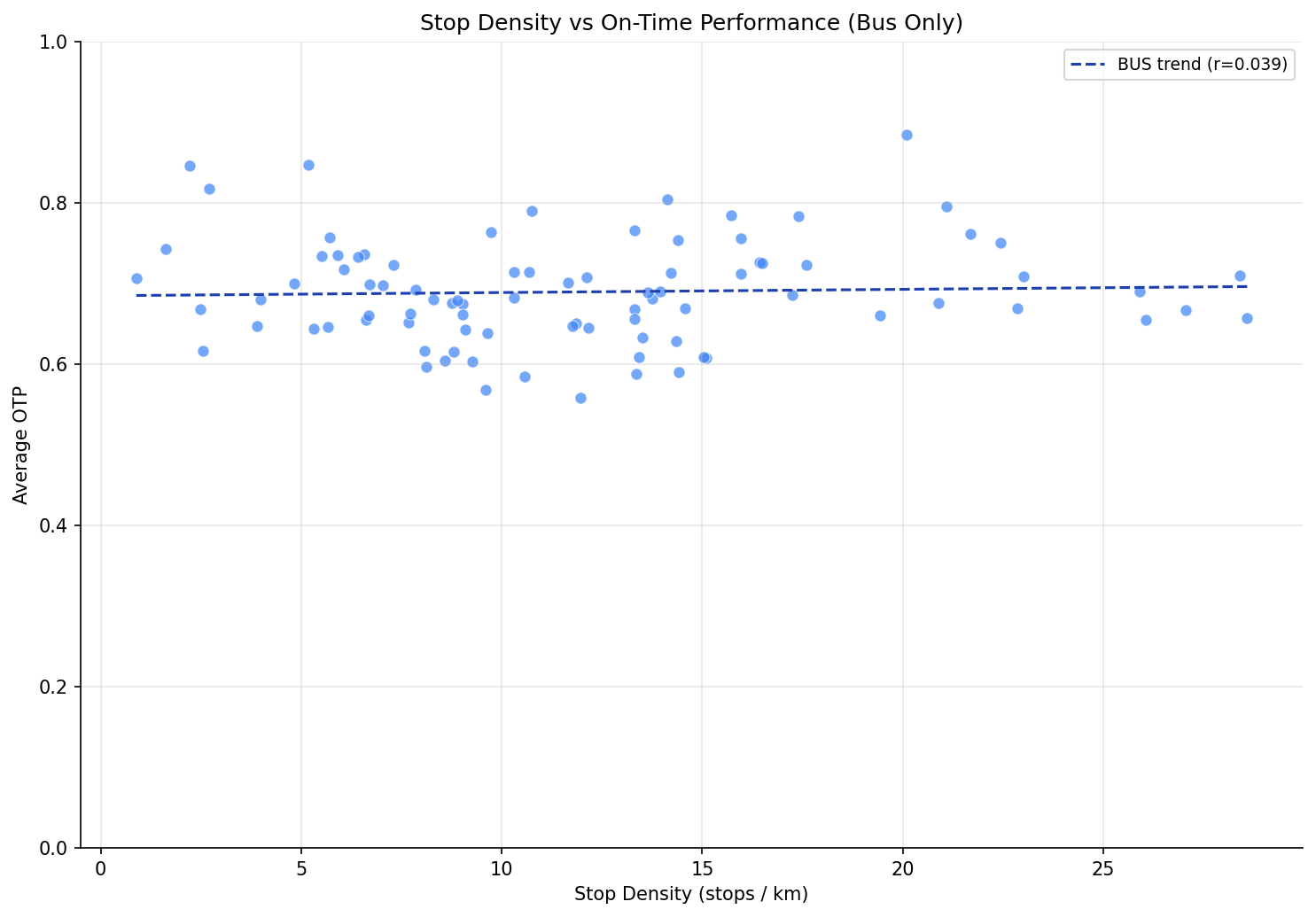
scatter plot of stop density vs OTP.
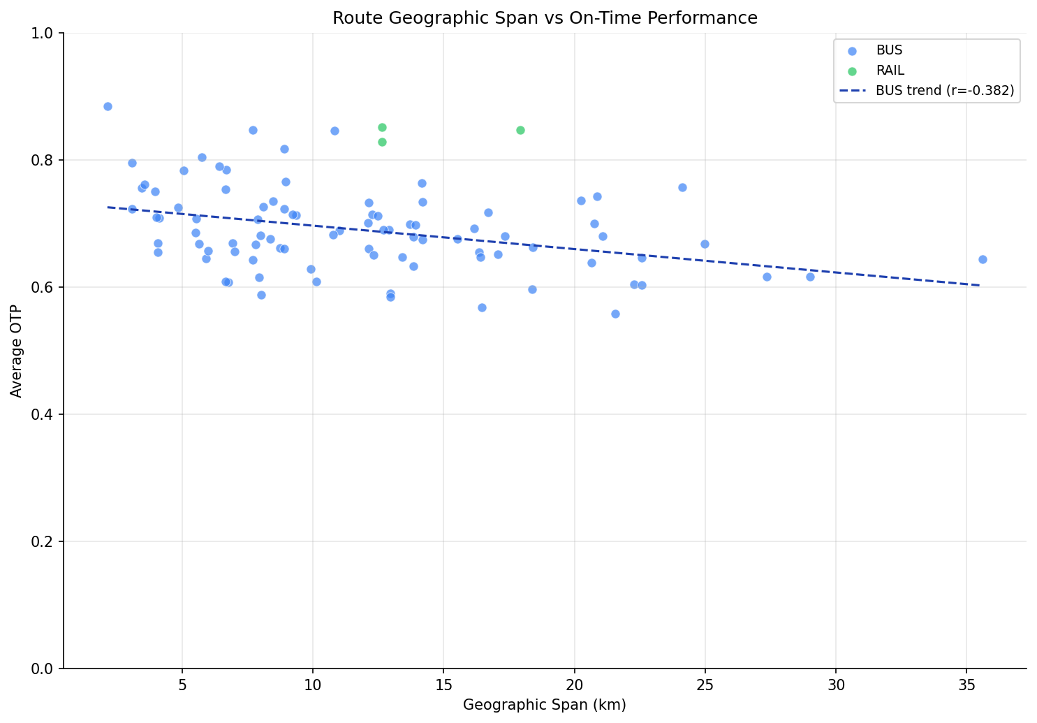
scatter plot of geographic span vs OTP.
No interactive outputs declared.
per-route span, stop density, stop count, avg OTP.
Preview CSV
Methods
Methods: Route Geographic Span vs OTP
Question
Does the geographic extent of a route predict on-time performance independently of stop count? Analysis 07 found stop count is the strongest OTP predictor (r = -0.53), but routes with many stops also tend to cover more distance. Disentangling the two could clarify whether the problem is "too many stops" or "too long a route."
Approach
- For each route, collect all stop coordinates from
route_stopsjoined tostops. - Compute geographic span as the maximum haversine distance between any pair of stops on the route (the diameter of the stop set in km).
- Compute stop density as stops per km of span, to capture how tightly packed stops are.
- Correlate span, stop density, and stop count separately with average OTP (Pearson and Spearman).
- Use partial correlation to test whether span predicts OTP after controlling for stop count, and vice versa.
- Scatter plots for span vs OTP and stop density vs OTP.
Data
| Name | Description | Source |
|---|---|---|
route_stops |
Links routes to stops | prt.db table |
stops |
Lat/lon coordinates | prt.db table |
otp_monthly |
Monthly OTP per route | prt.db table |
routes |
Mode classification | prt.db table |
Output
output/geographic_span.csv-- per-route span, stop density, stop count, avg OTPoutput/span_vs_otp.png-- scatter plot of geographic span vs OTPoutput/density_vs_otp.png-- scatter plot of stop density vs OTP
Source Code
|
Sources
| Name | Type | Why It Matters | Owner | Freshness | Caveat |
|---|---|---|---|---|---|
| otp_monthly | table | Primary analytical table used in this page's computations. | Produced by Data Ingestion. | Updated when the producing pipeline step is rerun. | Coverage depends on upstream source availability and ETL assumptions. |
Upstream sources (5)
|
|||||
| route_stops | table | Primary analytical table used in this page's computations. | Produced by Data Ingestion. | Updated when the producing pipeline step is rerun. | Coverage depends on upstream source availability and ETL assumptions. |
Upstream sources (5)
|
|||||
| routes | table | Primary analytical table used in this page's computations. | Produced by Data Ingestion. | Updated when the producing pipeline step is rerun. | Coverage depends on upstream source availability and ETL assumptions. |
Upstream sources (5)
|
|||||
| stops | table | Primary analytical table used in this page's computations. | Produced by Data Ingestion. | Updated when the producing pipeline step is rerun. | Coverage depends on upstream source availability and ETL assumptions. |
Upstream sources (5)
|
|||||
| numpy | dependency | Runtime dependency required for this page's pipeline or analysis code. | Open-source Python ecosystem maintainers. | Version pinned by project environment until dependency updates are applied. | Library updates may change behavior or defaults. |
| polars | dependency | Runtime dependency required for this page's pipeline or analysis code. | Open-source Python ecosystem maintainers. | Version pinned by project environment until dependency updates are applied. | Library updates may change behavior or defaults. |
| scipy | dependency | Runtime dependency required for this page's pipeline or analysis code. | Open-source Python ecosystem maintainers. | Version pinned by project environment until dependency updates are applied. | Library updates may change behavior or defaults. |