Analysis

07: Stop Count vs OTP

Core OTP Patterns

Coverage: 2019-01 to 2025-11 (from otp_monthly).

Built 2026-06-15 11:52 UTC · Commit e5cf673

Page Navigation

Analysis Navigation

Data Provenance

flowchart LR
  07_stop_count_vs_otp(["07: Stop Count vs OTP"])
  t_otp_monthly[("otp_monthly")] --> 07_stop_count_vs_otp
  01_data_ingestion[["Data Ingestion"]] --> t_otp_monthly
  u1_01_data_ingestion[/"data/routes_by_month.csv"/] --> 01_data_ingestion
  u2_01_data_ingestion[/"data/PRT_Current_Routes_Full_System_de0e48fcbed24ebc8b0d933e47b56682.csv"/] --> 01_data_ingestion
  u3_01_data_ingestion[/"data/Transit_stops_(current)_by_route_e040ee029227468ebf9d217402a82fa9.csv"/] --> 01_data_ingestion
  u4_01_data_ingestion[/"data/PRT_Stop_Reference_Lookup_Table.csv"/] --> 01_data_ingestion
  u5_01_data_ingestion[/"data/average-ridership/12bb84ed-397e-435c-8d1b-8ce543108698.csv"/] --> 01_data_ingestion
  t_route_stops[("route_stops")] --> 07_stop_count_vs_otp
  01_data_ingestion[["Data Ingestion"]] --> t_route_stops
  t_routes[("routes")] --> 07_stop_count_vs_otp
  01_data_ingestion[["Data Ingestion"]] --> t_routes
  d1_07_stop_count_vs_otp(("polars (lib)")) --> 07_stop_count_vs_otp
  d2_07_stop_count_vs_otp(("scipy (lib)")) --> 07_stop_count_vs_otp
  classDef page fill:#dbeafe,stroke:#1d4ed8,color:#1e3a8a,stroke-width:2px;
  classDef table fill:#ecfeff,stroke:#0e7490,color:#164e63;
  classDef dep fill:#fff7ed,stroke:#c2410c,color:#7c2d12,stroke-dasharray: 4 2;
  classDef file fill:#eef2ff,stroke:#6366f1,color:#3730a3;
  classDef api fill:#f0fdf4,stroke:#16a34a,color:#14532d;
  classDef pipeline fill:#f5f3ff,stroke:#7c3aed,color:#4c1d95;
  class 07_stop_count_vs_otp page;
  class t_otp_monthly,t_route_stops,t_routes table;
  class d1_07_stop_count_vs_otp,d2_07_stop_count_vs_otp dep;
  class u1_01_data_ingestion,u2_01_data_ingestion,u3_01_data_ingestion,u4_01_data_ingestion,u5_01_data_ingestion file;
  class 01_data_ingestion pipeline;

Findings

Findings: Stop Count vs OTP

Summary

There is a moderately strong negative correlation between the number of stops on a route and its average OTP. This finding holds for both all routes and bus-only analysis, ruling out Simpson's paradox as a confounder.

Key Numbers

All routes: Pearson r = -0.53 (p < 0.001, n = 92)
Bus only: Pearson r = -0.50 (p < 0.001, n = 89)
Bus only: Spearman r = -0.49 (p < 0.001)
Bus only, excluding 2 high-leverage routes (59, 77): Pearson r = -0.52 (p < 0.001, n = 87)
Routes with < 50 stops: typically 80%+ OTP
Routes with 150+ stops: typically below 60% OTP

Routes with fewer than 12 months of OTP data are excluded to avoid noisy averages from sparse observations.

Observations

The bus-only correlation (r = -0.50) is nearly as strong as the all-routes correlation (r = -0.53), confirming that the effect is not driven by the BUS/RAIL mode split (Simpson's paradox). Stop count predicts OTP within the bus mode alone.
The Spearman rank correlation (r = -0.49) is consistent with the Pearson, indicating the relationship is approximately monotonic without being driven by outliers or non-linearity.
Every stop adds dwell time (boarding/alighting), traffic signal delay, and schedule recovery risk. The cumulative effect is substantial.
Busway and rail routes tend to have fewer stops and dedicated right-of-way, giving them a double advantage.
Route 59 (Mon Valley) is the extreme stop-count route: 334 stops, 76 more than the next-highest route, winding through 17 Mon Valley municipalities. It is a high-leverage point on the scatter (leverage ~9x the average) and sits well above the trendline -- 0.69 OTP versus the ~0.56 the bus trend predicts at 334 stops. Despite the most stops in the system, it performs better than the model expects, likely because a dwell-heavy urban route carries a generously padded schedule. Its stop count is genuine, not a data artifact: every stop is served by the same single trip pattern (no branch-union inflation).
Route 77 (Penn Hills), at 258 stops, is the worst-performing high-stop route (0.56 OTP) -- the clearest illustration of the negative relationship. Unlike Route 59, it runs several branches, so its stop count is a union across patterns no single trip serves.
Excluding the two high-leverage routes (59 and 77) leaves the bus correlation essentially unchanged (r = -0.50 -> -0.52), so the headline relationship is not an artifact of the extreme-stop routes. Route 59 alone slightly masks the relationship: dropping just that point strengthens the bus Pearson to r = -0.55.

Implication

Stop consolidation -- reducing the number of stops on long routes -- is a common transit strategy for improving schedule adherence. This data strongly supports that approach for PRT's worst-performing routes.

Caveats

Correlation is not causation. Routes with many stops also tend to serve congested corridors, cover longer distances, and carry more passengers -- all of which independently affect OTP.
Temporal mismatch: Stop counts come from the current route_stops snapshot while OTP is averaged across all historical months (2019--2025). Routes that changed stop configurations during this period have a mismatch between their current stop count and earlier OTP observations. This is inherent to the available data and cannot be corrected without historical stop-count snapshots.

Validation

Surprising point investigated (checklist #5). Route 59's 334 stops -- 30% above the next-highest route -- was audited before being written up. In route_stops all 332 of its stops share an identical trips_7d of 162, indicating a single service pattern with no branch-union inflation; its stops span 17 contiguous Mon Valley municipalities. The count is a genuine long route, not a join error.
Outlier influence checked (checklist #5, #8). The bus regression has two high-leverage routes by the h > 3*(2/n) rule (59 and 77). The leverage-robustness check recomputes the bus Pearson with them removed (r = -0.52, n = 87); the headline finding is stable. Both extreme-stop routes are annotated on the chart.
Small-sample routes flagged (checklist #8). Routes with fewer than 12 months of OTP data are excluded (HAVING COUNT(*) >= 12).
Ecological framing (checklist #9). Results are route-level associations between stop count and average OTP; no individual-trip or individual-rider claims are made.

Review History

2026-02-11: RED-TEAM-REPORTS/2026-02-11-analyses-01-05-07-11.md — 6 issues (0 significant). Added 12-month minimum filter, temporal mismatch note in METHODS.md, all_n tracking, replaced manual regression with linregress, added min-n guard, updated METHODS.md for Pearson+Spearman.

Output

image stop_count_vs_otp.png
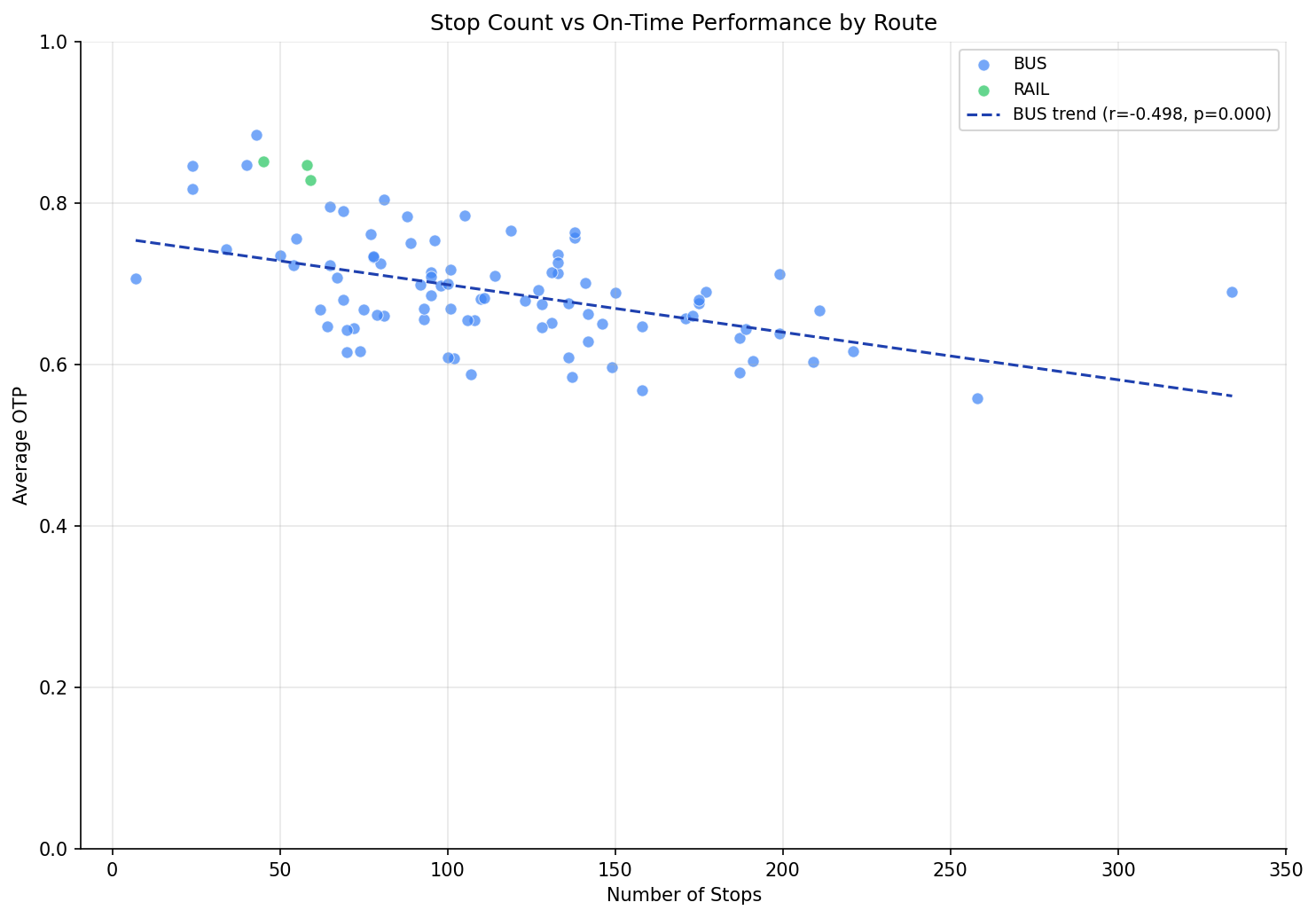
scatter plot with regression line.

No interactive outputs declared.

data stop_count_otp.csv

per-route stop count and average OTP.

Preview CSV

Expand to load preview.

Methods

Methods: Stop Count vs OTP

Question

Do routes with more stops have worse on-time performance? Each stop is another opportunity to fall behind schedule.

Approach

Count distinct stops per route from route_stops.
Compute average OTP per route from otp_monthly, requiring at least 12 months of data (HAVING COUNT(*) >= 12) to exclude routes with sparse observations.
Create a scatter plot of stop count vs average OTP, colored by mode.
Compute Pearson and Spearman correlation coefficients, both for all routes and for bus-only (to check for Simpson's paradox from mixing modes).
Fit a simple linear regression line (bus-only, via scipy.stats.linregress).
Leverage-robustness check: recompute the bus-only Pearson correlation after dropping high-leverage routes -- those whose regression leverage h = 1/n + (x - mean)^2 / Sxx exceeds 3 * (2/n), the standard rule of thumb for a two-parameter fit. This confirms the correlation is not an artifact of the few extreme-stop-count routes.
Annotate the two highest-stop-count routes (59 and 77) on the scatter so the influential points are visible to readers.

Note: Stop counts come from the current route_stops snapshot, while OTP is averaged across all historical months. Routes that changed stop configurations over time will have a mismatch between their current stop count and the OTP values from earlier periods.

Data

Name	Description	Source
`otp_monthly`	Monthly OTP per route	`prt.db` table
`route_stops`	Stop count per route	`prt.db` table
`routes`	Mode classification	`prt.db` table

Output

output/stop_count_otp.csv -- per-route stop count and average OTP
output/stop_count_vs_otp.png -- scatter plot with regression line

  Source Code
    
      
      """Scatter analysis of route stop count versus average on-time performance."""

import polars as pl
from scipy.stats import pearsonr

from prt_otp_analysis.common import analysis_dir, correlate_by_mode, mode_scatter, phase, query_to_polars, run_analysis, save_chart, save_csv, setup_plotting

OUT = analysis_dir(__file__)


def load_data() -> pl.DataFrame:
    """Load per-route stop counts, average OTP, and mode."""
    stop_counts = query_to_polars("""
        SELECT route_id, COUNT(DISTINCT stop_id) AS stop_count
        FROM route_stops
        GROUP BY route_id
    """)
    avg_otp = query_to_polars("""
        SELECT o.route_id, r.route_name, r.mode,
               AVG(o.otp) AS avg_otp, COUNT(*) AS months
        FROM otp_monthly o
        JOIN routes r ON o.route_id = r.route_id
        GROUP BY o.route_id
        HAVING COUNT(*) >= 12
    """)
    return avg_otp.join(stop_counts, on="route_id", how="inner")


def _high_leverage(x: list[float], cutoff_mult: float = 3.0) -> list[bool]:
    """Flag points whose simple-regression leverage exceeds the cutoff.

    Returns one bool per point. Leverage h_i = 1/n + (x_i - mean)^2 / Sxx;
    a point is flagged when h_i > cutoff_mult * (2/n), the standard rule of
    thumb for a two-parameter (slope + intercept) regression.
    """
    n = len(x)
    mean_x = sum(x) / n
    sxx = sum((xi - mean_x) ** 2 for xi in x)
    cutoff = cutoff_mult * 2 / n
    return [(1 / n + (xi - mean_x) ** 2 / sxx) > cutoff for xi in x]


def analyze(df: pl.DataFrame) -> tuple[pl.DataFrame, dict]:
    """Compute correlations plus a leverage-robustness check for bus routes.

    Adds ``bus_robust_*`` keys: the bus-only Pearson correlation recomputed
    after dropping high-leverage routes (the few extreme-stop-count points
    that disproportionately steer the trendline).
    """
    results = correlate_by_mode(df, "stop_count", "avg_otp")

    bus_df = df.filter(pl.col("mode") == "BUS")
    flagged = pl.Series(_high_leverage(bus_df["stop_count"].to_list()))
    robust_df = bus_df.filter(~flagged)
    r, p = pearsonr(robust_df["stop_count"].to_list(), robust_df["avg_otp"].to_list())
    results["bus_robust_pearson_r"] = float(r)
    results["bus_robust_pearson_p"] = float(p)
    results["bus_robust_n"] = robust_df.height
    results["bus_excluded_routes"] = bus_df.filter(flagged)["route_id"].to_list()
    return df, results


def make_chart(df: pl.DataFrame) -> None:
    """Generate scatter plot of stop count vs OTP with bus-only trendline."""
    plt = setup_plotting()
    fig, ax = plt.subplots(figsize=(10, 7))
    mode_scatter(ax, df, "stop_count", "avg_otp")
    for route in ("59", "77"):
        row = df.filter(pl.col("route_id") == route)
        if row.height:
            ax.annotate(
                f"Route {route}",
                (row["stop_count"][0], row["avg_otp"][0]),
                textcoords="offset points",
                xytext=(-9, 9),
                fontsize=8,
                ha="right",
                color="#1e3a5f",
            )
    ax.set_xlabel("Number of Stops")
    ax.set_ylabel("Average OTP")
    ax.set_title("Stop Count vs On-Time Performance by Route")
    ax.legend(fontsize=9)
    ax.set_ylim(0, 1)
    save_chart(fig, OUT / "stop_count_vs_otp.png")


@run_analysis(7, "Stop Count vs OTP")
def main() -> None:
    """Entry point: load data, analyze, chart, and save."""
    with phase("Loading data"):
        df = load_data()
        print(f"  {len(df)} routes with both stop count and OTP data")

    with phase("Analyzing"):
        df, results = analyze(df)
        print(f"  All routes:  Pearson r = {results['all_pearson_r']:.4f} (p = {results['all_pearson_p']:.4f}), n = {results['all_n']}")
        print(f"  Bus only:    Pearson r = {results['bus_pearson_r']:.4f} (p = {results['bus_pearson_p']:.4f})")
        print(f"               Spearman r = {results['bus_spearman_r']:.4f} (p = {results['bus_spearman_p']:.4f})")
        print(f"               n = {results['bus_n']} bus routes")
        excluded = ", ".join(results["bus_excluded_routes"]) or "none"
        print(f"  Bus robust:  Pearson r = {results['bus_robust_pearson_r']:.4f} (p = {results['bus_robust_pearson_p']:.4f}), n = {results['bus_robust_n']}")
        print(f"               high-leverage routes excluded: {excluded}")

    with phase("Saving CSV"):
        save_csv(df, OUT / "stop_count_otp.csv")

    with phase("Generating chart"):
        make_chart(df)


if __name__ == "__main__":
    main()

    

    

Sources

Name	Type	Why It Matters	Owner	Freshness	Caveat
otp_monthly	table	Primary analytical table used in this page's computations.	Produced by Data Ingestion.	Updated when the producing pipeline step is rerun.	Coverage depends on upstream source availability and ETL assumptions.
Upstream sources (5) file data/routes_by_month.csv — Monthly route OTP source table in wide format. file data/PRT_Current_Routes_Full_System_de0e48fcbed24ebc8b0d933e47b56682.csv — Current route metadata and mode classifications. file data/Transit_stops_(current)_by_route_e040ee029227468ebf9d217402a82fa9.csv — Current stop-to-route coverage and trip counts. file data/PRT_Stop_Reference_Lookup_Table.csv — Historical stop reference file with geography attributes. file data/average-ridership/12bb84ed-397e-435c-8d1b-8ce543108698.csv — Average ridership by route and month.
route_stops	table	Primary analytical table used in this page's computations.	Produced by Data Ingestion.	Updated when the producing pipeline step is rerun.	Coverage depends on upstream source availability and ETL assumptions.
Upstream sources (5) file data/routes_by_month.csv — Monthly route OTP source table in wide format. file data/PRT_Current_Routes_Full_System_de0e48fcbed24ebc8b0d933e47b56682.csv — Current route metadata and mode classifications. file data/Transit_stops_(current)_by_route_e040ee029227468ebf9d217402a82fa9.csv — Current stop-to-route coverage and trip counts. file data/PRT_Stop_Reference_Lookup_Table.csv — Historical stop reference file with geography attributes. file data/average-ridership/12bb84ed-397e-435c-8d1b-8ce543108698.csv — Average ridership by route and month.
routes	table	Primary analytical table used in this page's computations.	Produced by Data Ingestion.	Updated when the producing pipeline step is rerun.	Coverage depends on upstream source availability and ETL assumptions.
Upstream sources (5) file data/routes_by_month.csv — Monthly route OTP source table in wide format. file data/PRT_Current_Routes_Full_System_de0e48fcbed24ebc8b0d933e47b56682.csv — Current route metadata and mode classifications. file data/Transit_stops_(current)_by_route_e040ee029227468ebf9d217402a82fa9.csv — Current stop-to-route coverage and trip counts. file data/PRT_Stop_Reference_Lookup_Table.csv — Historical stop reference file with geography attributes. file data/average-ridership/12bb84ed-397e-435c-8d1b-8ce543108698.csv — Average ridership by route and month.
polars	dependency	Runtime dependency required for this page's pipeline or analysis code.	Open-source Python ecosystem maintainers.	Version pinned by project environment until dependency updates are applied.	Library updates may change behavior or defaults.
scipy	dependency	Runtime dependency required for this page's pipeline or analysis code.	Open-source Python ecosystem maintainers.	Version pinned by project environment until dependency updates are applied.	Library updates may change behavior or defaults.