Analysis

06: Seasonal Patterns

Core OTP Patterns

Coverage: 2019-01 to 2025-11 (from otp_monthly).

Built 2026-03-03 02:23 UTC · Commit defd5c8

Page Navigation

Analysis Navigation

Data Provenance

flowchart LR
  06_seasonal_patterns(["06: Seasonal Patterns"])
  t_otp_monthly[("otp_monthly")] --> 06_seasonal_patterns
  01_data_ingestion[["Data Ingestion"]] --> t_otp_monthly
  t_route_stops[("route_stops")] --> 06_seasonal_patterns
  01_data_ingestion[["Data Ingestion"]] --> t_route_stops
  t_routes[("routes")] --> 06_seasonal_patterns
  01_data_ingestion[["Data Ingestion"]] --> t_routes
  d1_06_seasonal_patterns(("numpy (lib)")) --> 06_seasonal_patterns
  d2_06_seasonal_patterns(("polars (lib)")) --> 06_seasonal_patterns
  classDef page fill:#dbeafe,stroke:#1d4ed8,color:#1e3a8a,stroke-width:2px;
  classDef table fill:#ecfeff,stroke:#0e7490,color:#164e63;
  classDef dep fill:#fff7ed,stroke:#c2410c,color:#7c2d12,stroke-dasharray: 4 2;
  classDef file fill:#eef2ff,stroke:#6366f1,color:#3730a3;
  classDef api fill:#f0fdf4,stroke:#16a34a,color:#14532d;
  classDef pipeline fill:#f5f3ff,stroke:#7c3aed,color:#4c1d95;
  class 06_seasonal_patterns page;
  class t_otp_monthly,t_route_stops,t_routes table;
  class d1_06_seasonal_patterns,d2_06_seasonal_patterns dep;
  class 01_data_ingestion pipeline;

Findings

Findings: Seasonal Patterns

Summary

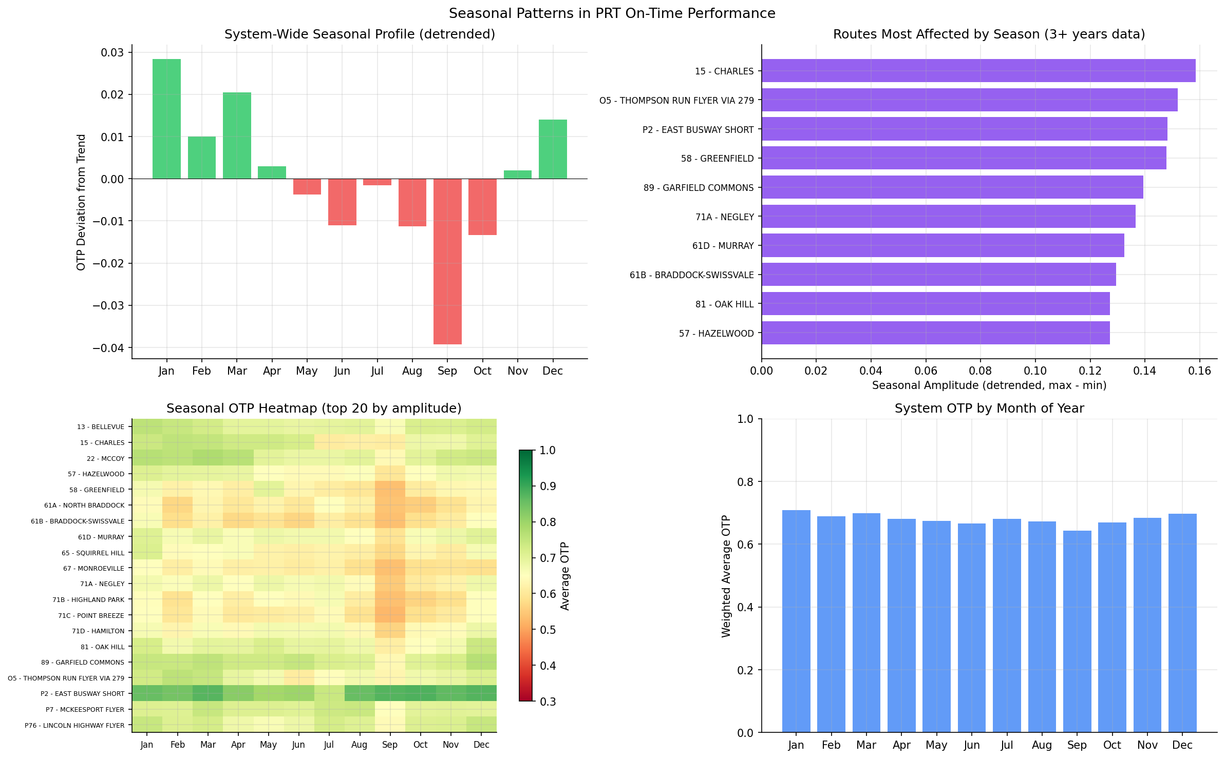
PRT shows a consistent seasonal cycle with winter months outperforming summer/fall. The system-wide seasonal swing is about 6.8 percentage points after detrending. 93 routes had sufficient data (3+ years) for route-level seasonal analysis.

System-Wide Seasonal Profile

Computed from a balanced panel of 93 routes (present in all 12 months-of-year) over complete calendar years (2019--2024).

Month	Weighted OTP	Deviation from Trend
January	70.8%	+2.8 pp (Best)
February	68.9%	+1.0 pp
March	69.9%	+2.1 pp
April	68.1%	+0.3 pp
May	67.4%	-0.4 pp
June	66.7%	-1.1 pp
July	68.1%	-0.2 pp
August	67.2%	-1.1 pp
September	64.4%	-3.9 pp (Worst)
October	66.9%	-1.3 pp
November	68.4%	+0.2 pp
December	69.6%	+1.4 pp

Methodology Note

Seasonal profiles are computed by first removing a 12-month centered rolling mean (trend), then averaging the detrended residuals by month-of-year. This ensures that long-term trends (e.g., the COVID dip) do not distort the seasonal pattern. Route-level analysis requires at least 3 years of data to ensure each month-of-year is represented multiple times.

Red-team corrections applied (2026-02-10):

Restricted to complete calendar years (2019-01 through 2024-12) to ensure every month-of-year has equal year coverage. Previously, December was missing 2025 data (the worst-performing year), inflating its seasonal average.
Used a balanced panel of routes present in all 12 months-of-year for the system-wide profile. This excluded 5 routes: 3 winter-only routes with very high OTP (37 Castle Shannon 81%, 42 Potomac 83%, RLSH Red Line Shuttle 98%) and 2 with other gaps (53 Homestead Park, SWL). Their inclusion previously inflated winter averages.
Note: trips_7d weighting is a static snapshot and may not reflect historical service levels. The seasonal pattern holds in both weighted and unweighted averages, so the core finding is robust to weighting choice.

Most Seasonally Affected Routes (detrended)

Route	Seasonal Amplitude
15 - Charles	15.8%
O5 - Thompson Run Flyer via 279	15.2%
P2 - East Busway Short	14.8%

Observations

The winter advantage is somewhat counterintuitive -- one might expect snow and ice to worsen OTP. Possible explanations: lower ridership reduces dwell time; fewer construction detours; school breaks reduce congestion.
September is consistently the worst month (-3.9 pp from trend), possibly due to the return of school-year traffic and late-summer construction.
After applying the balanced panel filter and complete-years restriction, the seasonal pattern persists with minimal change in magnitude, confirming it is a genuine operational pattern rather than a data artifact.
Most routes have a seasonal amplitude under 15%. The heatmap of the top 20 routes shows no single month dominates as "worst" across all routes -- the pattern varies, though fall months are generally weaker.

Caveats

Seasonal decomposition uses a centered moving-average method to remove trend, not a formal STL decomposition. Results are directionally correct but assume additive seasonality.
Only 6 years of complete data (2019--2024) means each month-of-year average is based on ~6 detrended observations, limiting statistical power.
The trips_7d weighting reflects a single point-in-time snapshot of service frequency, not historical values. Route frequencies likely changed over the study period (especially during COVID).

Review History

2026-02-10: RED-TEAM-REPORTS/2026-02-10-analysis-06-seasonal-patterns.md — 4 issues (2 moderate). Balanced panel and complete-years restrictions applied; core finding confirmed.

Output

No interactive outputs declared.

data seasonal_patterns.csv

month-of-year seasonal profile per route.

Preview CSV

Expand to load preview.

Methods

Methods: Seasonal Patterns

Question

Do PRT routes exhibit consistent seasonal OTP patterns? Are summer or winter months systematically better or worse?

Approach

Restrict to complete calendar years (2019--2024) to ensure every month-of-year has equal year coverage.
Use a balanced panel of routes present in all 12 months-of-year for the system-wide profile, preventing compositional bias from seasonal or short-lived routes.
Compute a system-wide seasonal profile by averaging across balanced-panel routes (trip-weighted).
Measure seasonal amplitude: max(month-of-year avg) - min(month-of-year avg) per route.
Decompose into trend + seasonal + residual using a moving-average approach:
1. Trend = 12-month centered rolling mean
2. Seasonal = month-of-year mean of (OTP - trend)
3. Residual = OTP - trend - seasonal
Rank routes by seasonal amplitude to identify those most affected by seasons.
Route-level analysis requires at least 3 years of data (36 months) for reliable seasonal estimates.

Data

Name	Description	Source
`otp_monthly`	Monthly OTP per route	`prt.db` table
`route_stops`	Trip counts for weighting	`prt.db` table
`routes`	Route metadata	`prt.db` table

Output

output/seasonal_patterns.csv -- month-of-year seasonal profile per route
output/seasonal_patterns.png -- seasonal decomposition charts

Sources

Name	Type	Why It Matters	Owner	Freshness	Caveat
otp_monthly	table	Primary analytical table used in this page's computations.	Produced by Data Ingestion.	Updated when the producing pipeline step is rerun.	Coverage depends on upstream source availability and ETL assumptions.
route_stops	table	Primary analytical table used in this page's computations.	Produced by Data Ingestion.	Updated when the producing pipeline step is rerun.	Coverage depends on upstream source availability and ETL assumptions.
routes	table	Primary analytical table used in this page's computations.	Produced by Data Ingestion.	Updated when the producing pipeline step is rerun.	Coverage depends on upstream source availability and ETL assumptions.
numpy	dependency	Runtime dependency required for this page's pipeline or analysis code.	Open-source Python ecosystem maintainers.	Version pinned by project environment until dependency updates are applied.	Library updates may change behavior or defaults.
polars	dependency	Runtime dependency required for this page's pipeline or analysis code.	Open-source Python ecosystem maintainers.	Version pinned by project environment until dependency updates are applied.	Library updates may change behavior or defaults.