Analysis

53 - Near-Side vs. Far-Side Stop Placement

Coverage: 2019-01 to 2025-11 (from otp_monthly).

Built 2026-06-15 11:52 UTC · Commit e5cf673

Page Navigation

Analysis Navigation

Data Provenance

flowchart LR
  53_stop_signal_placement(["53 - Near-Side vs. Far-Side Stop Placement"])
  f1_53_stop_signal_placement[/"data/GTFS/stops.txt"/] --> 53_stop_signal_placement
  f2_53_stop_signal_placement[/"data/GTFS/trips.txt"/] --> 53_stop_signal_placement
  f3_53_stop_signal_placement[/"data/GTFS/stop_times.txt"/] --> 53_stop_signal_placement
  f4_53_stop_signal_placement[/"data/GTFS/shapes.txt"/] --> 53_stop_signal_placement
  f5_53_stop_signal_placement[/"data/osm-signals/traffic_signals_raw.json"/] --> 53_stop_signal_placement
  t_otp_monthly[("otp_monthly")] --> 53_stop_signal_placement
  01_data_ingestion[["Data Ingestion"]] --> t_otp_monthly
  u1_01_data_ingestion[/"data/routes_by_month.csv"/] --> 01_data_ingestion
  u2_01_data_ingestion[/"data/PRT_Current_Routes_Full_System_de0e48fcbed24ebc8b0d933e47b56682.csv"/] --> 01_data_ingestion
  u3_01_data_ingestion[/"data/Transit_stops_(current)_by_route_e040ee029227468ebf9d217402a82fa9.csv"/] --> 01_data_ingestion
  u4_01_data_ingestion[/"data/PRT_Stop_Reference_Lookup_Table.csv"/] --> 01_data_ingestion
  u5_01_data_ingestion[/"data/average-ridership/12bb84ed-397e-435c-8d1b-8ce543108698.csv"/] --> 01_data_ingestion
  t_stop_signals[("stop_signals")] --> 53_stop_signal_placement
  15_stop_signals[["PRT Stop-Signal Classification ETL"]] --> t_stop_signals
  u1_15_stop_signals[/"data/prt-stop-signals/bus_stops_with_signals_2602.xlsx"/] --> 15_stop_signals
  t_route_stops[("route_stops")] --> 53_stop_signal_placement
  01_data_ingestion[["Data Ingestion"]] --> t_route_stops
  d1_53_stop_signal_placement(("analyses/51_traffic_signals_otp (lib)")) --> 53_stop_signal_placement
  classDef page fill:#dbeafe,stroke:#1d4ed8,color:#1e3a8a,stroke-width:2px;
  classDef table fill:#ecfeff,stroke:#0e7490,color:#164e63;
  classDef dep fill:#fff7ed,stroke:#c2410c,color:#7c2d12,stroke-dasharray: 4 2;
  classDef file fill:#eef2ff,stroke:#6366f1,color:#3730a3;
  classDef api fill:#f0fdf4,stroke:#16a34a,color:#14532d;
  classDef pipeline fill:#f5f3ff,stroke:#7c3aed,color:#4c1d95;
  class 53_stop_signal_placement page;
  class t_otp_monthly,t_route_stops,t_stop_signals table;
  class d1_53_stop_signal_placement dep;
  class f1_53_stop_signal_placement,f2_53_stop_signal_placement,f3_53_stop_signal_placement,f4_53_stop_signal_placement,f5_53_stop_signal_placement,u1_01_data_ingestion,u1_15_stop_signals,u2_01_data_ingestion,u3_01_data_ingestion,u4_01_data_ingestion,u5_01_data_ingestion file;
  class 01_data_ingestion,15_stop_signals pipeline;

Findings

Findings: Near-Side vs. Far-Side Stop Placement

Summary

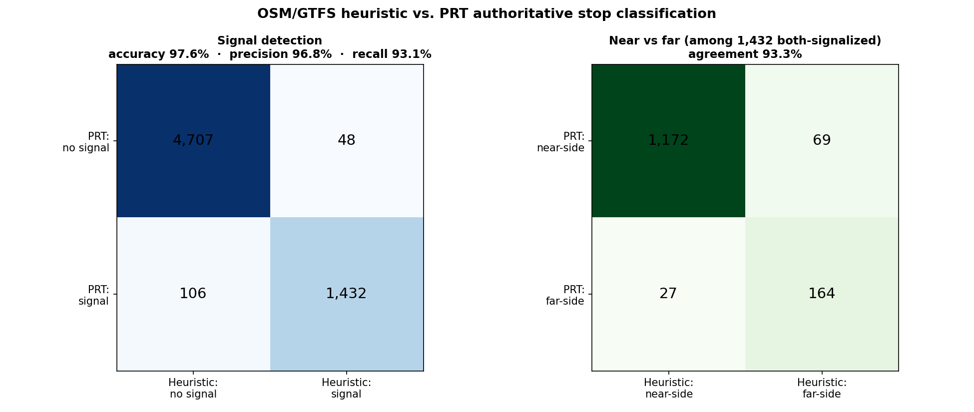
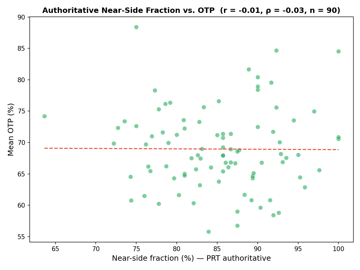
PRT bus stops at signalized intersections are overwhelmingly placed on the near side — before the traffic light in the direction of travel. PRT's own authoritative stop records (the stop_signals table, supplied by PRT) classify 1,539 stops as signalized, of which 86% are near-side (1,320) and only 14% are far-side (219); a further 66 are busway/BRT and the remaining 4,701 bus stops are not at a signal. An independent OSM/GTFS heuristic built from scratch (Steps 1–5) agreed with these authoritative labels on 97.6% of stops for signal detection and 93.3% for near-vs-far — validating the method that earlier analyses relied on. Re-running the route-level OTP test on the authoritative labels leaves the result null (r = −0.01, p = 0.95, n = 90): whether a route's stops are more near-side or far-side has no measurable association with how on-time it runs, driven by severe range restriction (almost every route is 64–100% near-side).

Key Numbers

Authoritative (PRT stop_signals)

  • 6,306 PRT bus stops, of which 1,539 are at a traffic signal (1,320 near-side + 219 far-side), 66 busway/BRT, 4,701 no signal.
  • Among signalized stops: 85.8% near-side, 14.2% far-side.
  • 90 routes had ≥ 3 authoritative signalized stops and OTP data.
  • Authoritative near-side fraction by route ranges 64% to 100% (median 86%).
  • Authoritative OTP correlation: r = −0.01 (p = 0.95), ρ = −0.03 (p = 0.80) — null.

Heuristic validation (OSM/GTFS vs. PRT, 6,293 stops in both)

  • Signal detection: accuracy 97.6%, precision 96.8%, recall 93.1% (TP 1,432 · FP 48 · FN 106 · TN 4,707). The heuristic misses ~7% of signalized stops, mostly where OSM has no signal node within 50 m.
  • Near vs. far: 93.3% agreement (1,336 / 1,432). The heuristic slightly over-calls far-side (68 truly-near labelled far vs. 27 truly-far labelled near).

Heuristic, for reference (OSM/GTFS only)

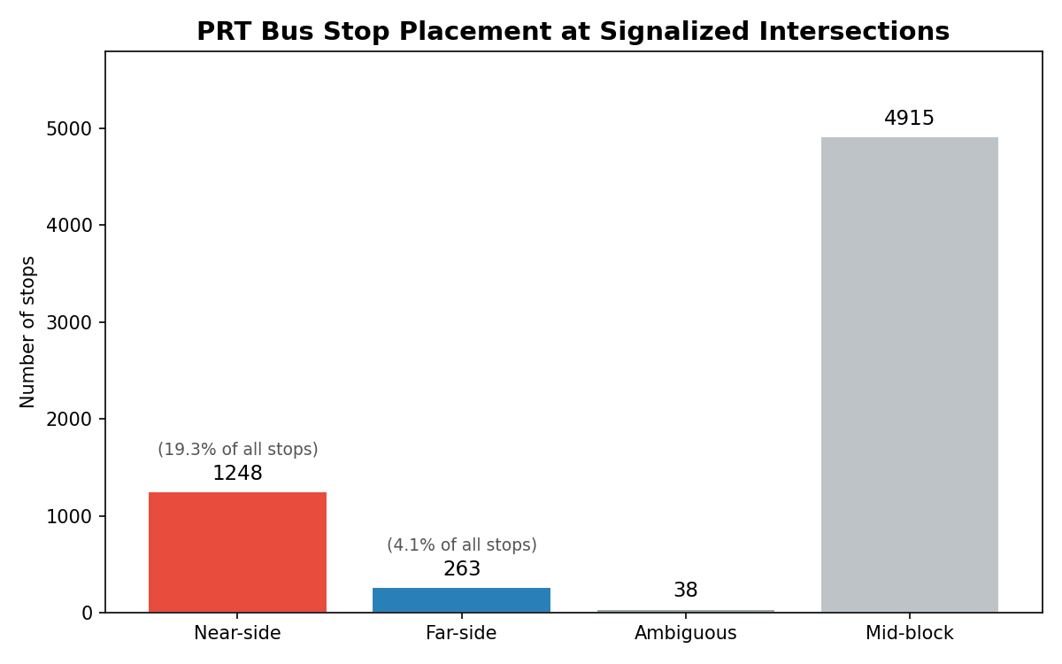
  • 1,549 stops within 50 m of an OSM signal: 1,248 near-side (83%), 263 far-side (17%), 38 ambiguous; 4,915 mid-block.
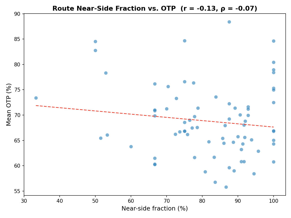
  • Heuristic OTP correlation: r = −0.13 (p = 0.26), ρ = −0.07 — not significant.

Observations

  • The OSM/GTFS heuristic is validated. Against PRT's authoritative records, the from-scratch geometric method correctly identifies signalized stops 97.6% of the time and gets near-vs-far right 93.3% of the time. This retroactively supports the OSM-derived signal metrics used in Analysis 51 and the placement classification used here and in Analysis 54 — the proxy was sound. Where it errs, it is mostly conservative (106 signalized stops missed because OSM lacks a node within 50 m), so the heuristic slightly under-counts signal exposure.
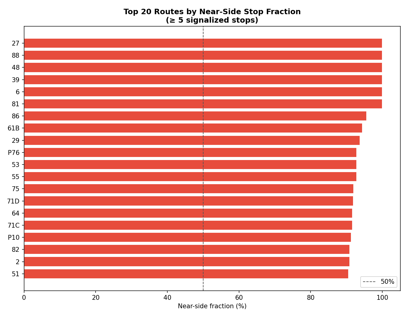
  • Near-side is the overwhelming default. Across nearly every PRT route, buses stop before the signal, not after. The near-side fraction drops below 70% only for a handful of routes. This is consistent with older US transit practice — near-side stops were historically preferred because the bus can open doors while waiting for a red, allowing simultaneous boarding/signal-wait. Modern transit operations guidance favors far-side because the bus clears the intersection before stopping (no double-stop), benefits from a rolling start on the green, and keeps the bus out of the box during the red.
  • The OTP correlation is weak and non-significant. This does not mean near-side placement is harmless — the mechanism is plausible, and the lack of signal is best explained by two factors: (1) near-side fraction varies little across routes (most routes are 80–100% near-side, offering little statistical leverage), and (2) the Analysis 51 structural predictors (signal density, stop count, route length) already absorb most of the variance, leaving little for placement type to explain at the route level. A stop-level or trip-level analysis with actual dwell/departure data would be needed to test the mechanism directly.
  • Far-side stops cluster on newer or rebuilt corridors. Routes with higher far-side fractions (near-side fraction ~33–50%) tend to be routes that have seen more recent infrastructure investment or run on busier arterials where signals were added or retimed more recently. This is not formally tested here.
  • Most stops are mid-block. 76% of PRT stops have no signal within 50 m. Pittsburgh's dense, hilly street grid means many stops are in the middle of short block faces, away from intersections — reducing the operational relevance of near/far placement for the majority of the network.

Discussion

This is a descriptive analysis: it establishes what the current placement mix looks like, not whether changing placement would improve OTP. The practical implication is that if PRT or City of Pittsburgh were to invest in stop relocation or signal retiming as part of a transit priority program, the near-side-to-far-side conversion case is strongest on routes where (a) near-side fraction is high, (b) signal density is high (Analysis 51), and (c) OTP is already low — the dense East End local routes (71B, 81, 83, 82) score on all three dimensions.

The Analysis 51 finding that signal density predicts OTP independently of stop count remains the more actionable result. Near-side placement adds a plausible incremental delay per stop, but the bigger issue is that these routes encounter many signals at all — each one adding a stochastic cycle wait regardless of whether the stop is before or after it.

The weak OTP correlation here (and in the follow-up Analysis 54) should not be read as evidence that placement type is irrelevant. The fundamental obstacle is range restriction: with 80–100% near-side fraction on most routes, there is not enough cross-route variance to detect an effect at the route level even if one exists at the stop level. The right test — a paired comparison of otherwise identical near-side and far-side stops using stop-level arrival time data — is not possible with the current data.

Caveats

  • Single-direction classification. Each stop is classified using its canonical shape (most-served direction). A stop serving both inbound and outbound trips may be near-side in one direction and far-side in the other. The classification reflects the dominant direction only.
  • OSM signal proximity ≠ same-street signal. The 50 m match finds the nearest signal node, which may be on a crossing street rather than the bus's travel direction. In practice this affects corner stops where a signal governs the perpendicular road rather than the arterial the bus runs on.
  • OSM signal coverage is crowd-sourced. The 2,820 county-wide signals are in the expected range, but completeness is higher in the City of Pittsburgh than in outer suburbs. Suburban stops near signals may appear as mid-block simply due to incomplete OSM coverage.
  • Lat/lon projection. Shape projection uses Shapely on geographic coordinates (not projected), which is approximate. For the purpose of determining order along a route (near vs. far), this approximation is acceptable; the ambiguous threshold (5 m) filters co-located cases.
  • Ecological framing. All OTP results are route-level associations. No trip-level or rider-level causal claims are made.

Validation

  1. Data source verified. Stops from data/GTFS/stops.txt (6,464 bus stops after excluding 4 station nodes). Signals from data/osm-signals/traffic_signals_raw.json (2,820 nodes; matches Analysis 51 count). OTP from otp_monthly table, same query as prior analyses.
  2. Scope match. GTFS stops and OSM signals both cover Allegheny County. OTP is averaged across all months per route (no temporal filter applied — consistent with route-level correlation approach).
  3. Null handling. Stops without a canonical shape (no stop_times match) are excluded from near/far classification but counted as mid-block in system-wide totals. The 37 ambiguous stops are excluded from the near/far ratio and from the OTP correlation.
  4. Aggregate sanity check. Total signalized stops (1,549) is 24% of all stops — plausible given that many PRT stops are on block faces away from intersections. 83% near-side is high but consistent with literature on older US bus networks. Far-side fraction (17%) is in the range reported for networks that have not undergone systematic stop placement policy.
  5. Surprising result check. The 83% near-side finding is striking but explainable: PRT's stop infrastructure largely predates modern far-side guidance, and Pittsburgh's grid makes mid-block placement common, so intersection stops disproportionately reflect legacy near-side siting.
  6. Direction of effects. The OTP correlation is in the expected direction (negative: more near-side → slightly lower OTP), even if non-significant. A positive coefficient would have been a red flag.
  7. Cross-validated against authoritative source. PRT's stop_signals table (pipeline 15) provides ground-truth labels. The heuristic's aggregate split (83% near-side) is within 3 pp of the authoritative split (86%), and per-stop agreement is high (97.6% detection, 93.3% near/far). The headline near/far split and OTP correlation reported above use the authoritative labels; the heuristic is retained only for the validation comparison. Join is on the shared stop_code; the GTFS and PRT internal stop_id namespaces differ (GTFS numeric vs. PRT alpha-prefixed), so joining on stop_id would silently match nothing — a verified gotcha.

Output
Methods

Methods: Near-Side vs. Far-Side Stop Placement

Question

Are PRT bus stops placed before (near-side) or after (far-side) traffic signals at signalized intersections? What fraction of stops at signals are near-side vs. far-side, and does placement correlate with route-level OTP?

Approach

Step 1 — Match stops to nearby signals

For every GTFS stop, find all OSM traffic signals within a 50 m radius. A stop with no signal within 50 m is classified as "mid-block" and excluded from the near/far analysis. The 50 m threshold captures stops set back slightly from the crosswalk box while avoiding picking up the next intersection (typical Pittsburgh block face is 80–120 m).

Step 2 — Assign each stop to a canonical route shape

A stop may serve many trips. Pick the single GTFS shape that visits the stop the most times (stop_timestripsshapes). Use that shape to infer the direction of travel through the stop.

Step 3 — Determine near-side vs. far-side via shape projection

Project both the stop coordinate and the nearby signal coordinate onto the canonical shape polyline using the Shapely project method (returns distance along the line).

  • Near-side: stop's along-shape position < signal's along-shape position (stop comes first in the direction of travel → bus stops, boards, then waits for the light).
  • Far-side: stop's along-shape position > signal's along-shape position (bus clears the intersection, then stops to board).
  • Ambiguous: stop and signal project to within 5 m of each other along the shape (essentially co-located; excluded from near/far counts).

Step 4 — Aggregate and summarize

  • System-wide fraction: near-side / far-side / mid-block counts.
  • By route: fraction of signalized stops that are near-side; join to route OTP from otp_monthly to test for correlation.
  • By neighborhood / planning district (optional, if a spatial join to a neighborhood GeoJSON is available).

Step 5 — OTP correlation

Compute Pearson r and Spearman ρ between each route's near-side fraction and its mean OTP. Transit-operations theory predicts near-side stops are worse for OTP (bus must stop twice — once for passengers, once for the light), so a negative correlation between near-side fraction and OTP is the expected sign.

Step 6 — Validate against PRT's authoritative classification

PRT supplied an authoritative per-stop signal classification (the stop_signals table, built by pipeline/15_stop_signals/). The GTFS heuristic above is compared against it stop-by-stop on the shared stop_code key:

  • Signal detection — a 2×2 confusion matrix of heuristic "signalized" (near/far) vs. PRT "has signal", reporting precision, recall, and accuracy.
  • Near vs. far — among stops both sources call signalized, the agreement rate and a 2×2 near/far confusion matrix.

The route-level OTP correlation (Step 5) is then re-run on the authoritative near/far labels (joining stop_signalsroute_stopsotp_monthly), so the headline OTP result no longer depends on the OSM proxy.

Data

Source How used
data/GTFS/stops.txt Stop lat/lon and stop_code (join key to authoritative labels)
data/GTFS/shapes.txt Route shape polylines for direction-of-travel projection
data/GTFS/stop_times.txt Links stops → trips for canonical shape assignment
data/GTFS/trips.txt Links trips → shape_id
data/osm-signals/traffic_signals_raw.json Signal lat/lon (2,820 OSM nodes) — heuristic only
stop_signals table in prt.db PRT authoritative per-stop signal class (validation + authoritative re-run)
route_stops table in prt.db Stop → route mapping for authoritative route-level aggregation
otp_monthly table in prt.db Route mean OTP for correlation step

Stops are filtered to bus stops only (exclude light-rail stations whose right-of-way geometry differs fundamentally from street stops).

Output

  • output/stop_classifications.csv — one row per stop; columns: stop_id, stop_name, lat, lon, classification (near_side/far_side/mid_block/ambiguous), nearest_signal_distance_m, shape_id
  • output/route_summary.csv — one row per route; near_side_count, far_side_count, mid_block_count, near_side_fraction, mean_otp
  • output/system_summary.png — bar chart: system-wide stop classification breakdown
  • output/nearside_vs_otp.png — scatter plot: route near-side fraction vs. mean OTP (with regression line)
  • output/top_nearside_routes.png — ranked bar chart of routes by near-side fraction
  • output/heuristic_vs_authoritative.csv — per-stop comparison of the GTFS heuristic label vs. PRT's authoritative class (join on stop_code)
  • output/validation_confusion.png — confusion matrices: signal detection (left) and near vs. far (right), heuristic vs. PRT
  • output/authoritative_route_summary.csv — per-route near/far counts and mean OTP using PRT authoritative labels
  • output/authoritative_nearside_vs_otp.png — scatter: route near-side fraction (authoritative) vs. mean OTP

Source Code

"""Classify PRT bus stops as near-side or far-side relative to nearby traffic signals."""

from __future__ import annotations

import json
from pathlib import Path

import matplotlib.pyplot as plt
import numpy as np
import polars as pl
from scipy.spatial import cKDTree
from scipy.stats import pearsonr, spearmanr
from shapely.geometry import LineString, Point

from prt_otp_analysis.common import get_db

ANALYSIS_DIR = Path(__file__).parent
OUTPUT_DIR = ANALYSIS_DIR / "output"
GTFS_DIR = Path(__file__).parent.parent.parent / "data" / "GTFS"
OSM_SIGNALS_PATH = (
    Path(__file__).parent.parent.parent / "data" / "osm-signals" / "traffic_signals_raw.json"
)

# Tuning constants
SIGNAL_RADIUS_M = 50.0       # max stop-to-signal distance to count as "at an intersection"
AMBIGUOUS_THRESHOLD_M = 5.0  # stops and signals this close along-shape are ambiguous
DEGREES_PER_METER = 1 / 111_320  # approximate; used for KD-tree radius conversion


def load_signals() -> np.ndarray:
    """Return (N, 2) array of signal [lat, lon]."""
    with open(OSM_SIGNALS_PATH) as f:
        raw = json.load(f)
    return np.array([[e["lat"], e["lon"]] for e in raw])


def load_stops() -> pl.DataFrame:
    """Load GTFS stops, excluding the 4 explicit station nodes."""
    return (
        pl.read_csv(
            GTFS_DIR / "stops.txt",
            schema_overrides={"stop_id": pl.Utf8, "stop_code": pl.Int64},
        )
        .filter(pl.col("location_type").is_null())
        .select(["stop_id", "stop_code", "stop_name", "stop_lat", "stop_lon"])
    )


def load_authoritative() -> pl.DataFrame:
    """Load PRT's authoritative per-stop signal classification, keyed by stop_code.

    Returns columns: stop_code, auth_class ('none'|'nearside'|'farside'|'busway'),
    auth_has_signal (1 if at a non-busway signal). The PRT spreadsheet and GTFS share
    the stop_code key; their internal stop_id namespaces differ.
    """
    db = get_db()
    rows = db.execute(
        "SELECT stop_code, signal_class, has_signal FROM stop_signals"
    ).fetchall()
    return pl.DataFrame(
        {
            "stop_code": [int(r[0]) for r in rows],
            "auth_class": [r[1] for r in rows],
            "auth_has_signal": [int(r[2]) for r in rows],
        },
        schema={"stop_code": pl.Int64, "auth_class": pl.Utf8, "auth_has_signal": pl.Int64},
    )


def load_canonical_shapes() -> pl.DataFrame:
    """For each stop, return the shape_id used by the most trips.

    Returns a DataFrame with columns: stop_id, shape_id, route_id.
    """
    trips_df = pl.read_csv(
        GTFS_DIR / "trips.txt",
        schema_overrides={
            "trip_id": pl.Utf8,
            "shape_id": pl.Utf8,
            "route_id": pl.Utf8,
            "service_id": pl.Utf8,
        },
    ).select(["trip_id", "shape_id", "route_id"])

    stop_times_df = pl.read_csv(
        GTFS_DIR / "stop_times.txt",
        schema_overrides={"trip_id": pl.Utf8, "stop_id": pl.Utf8},
    ).select(["trip_id", "stop_id"])

    return (
        stop_times_df
        .join(trips_df, on="trip_id")
        .group_by(["stop_id", "shape_id", "route_id"])
        .agg(pl.len().alias("trip_count"))
        .sort("trip_count", descending=True)
        .unique(subset=["stop_id"], keep="first")
        .select(["stop_id", "shape_id", "route_id"])
    )


def build_shape_lines(shape_ids: set[str]) -> dict[str, LineString]:
    """Load GTFS shapes and return a dict of shape_id → Shapely LineString."""
    shapes_df = (
        pl.read_csv(
            GTFS_DIR / "shapes.txt",
            schema_overrides={"shape_id": pl.Utf8},
        )
        .filter(pl.col("shape_id").is_in(shape_ids))
        .sort(["shape_id", "shape_pt_sequence"])
    )

    lines: dict[str, LineString] = {}
    for (shape_id,), group in shapes_df.group_by("shape_id"):
        coords = list(zip(group["shape_pt_lon"].to_list(), group["shape_pt_lat"].to_list()))
        if len(coords) >= 2:
            lines[shape_id] = LineString(coords)
    return lines


def classify_stop(
    stop_lat: float,
    stop_lon: float,
    signal_lat: float,
    signal_lon: float,
    shape_line: LineString,
) -> str:
    """Return 'near_side', 'far_side', or 'ambiguous'."""
    stop_pt = Point(stop_lon, stop_lat)
    signal_pt = Point(signal_lon, signal_lat)

    stop_pos = shape_line.project(stop_pt)
    signal_pos = shape_line.project(signal_pt)

    delta_deg = signal_pos - stop_pos
    delta_m = delta_deg / DEGREES_PER_METER
    if abs(delta_m) <= AMBIGUOUS_THRESHOLD_M:
        return "ambiguous"
    return "near_side" if delta_deg > 0 else "far_side"


def main() -> None:
    OUTPUT_DIR.mkdir(exist_ok=True)

    print("Loading stops and signals…")
    stops_df = load_stops()
    signals = load_signals()  # shape (N, 2): [lat, lon]

    # Build KD-tree on signals (lat/lon degrees)
    tree = cKDTree(signals)
    stop_coords = stops_df.select(["stop_lat", "stop_lon"]).to_numpy()
    radius_deg = SIGNAL_RADIUS_M * DEGREES_PER_METER
    nearest_dists, nearest_idxs = tree.query(stop_coords, k=1, distance_upper_bound=radius_deg)

    has_signal = nearest_dists < radius_deg
    safe_idxs = nearest_idxs.clip(0, len(signals) - 1)
    signal_lat_col = np.where(has_signal, signals[safe_idxs, 0], np.nan)
    signal_lon_col = np.where(has_signal, signals[safe_idxs, 1], np.nan)
    dist_m_col = np.where(has_signal, nearest_dists / DEGREES_PER_METER, np.nan)

    stops_df = stops_df.with_columns([
        pl.Series("has_signal", has_signal),
        pl.Series("signal_lat", signal_lat_col),
        pl.Series("signal_lon", signal_lon_col),
        pl.Series("signal_dist_m", dist_m_col),
    ])
    print(f"  {has_signal.sum()} of {len(stops_df)} stops have a signal within {SIGNAL_RADIUS_M} m")

    print("Loading canonical shapes…")
    canonical_df = load_canonical_shapes()
    stops_df = stops_df.join(canonical_df, on="stop_id", how="left")

    classifiable_df = stops_df.filter(
        pl.col("has_signal") & pl.col("shape_id").is_not_null()
    )
    print(f"  {len(classifiable_df)} stops are classifiable (signal + shape)")

    print("Building shape geometries…")
    needed_ids = set(classifiable_df["shape_id"].to_list())
    shape_lines = build_shape_lines(needed_ids)
    print(f"  Loaded {len(shape_lines)} shape polylines")

    print("Classifying stops…")
    classifications: list[str] = []
    for row in classifiable_df.iter_rows(named=True):
        sid = row["shape_id"]
        if sid not in shape_lines:
            classifications.append("no_shape")
            continue
        classifications.append(
            classify_stop(
                row["stop_lat"], row["stop_lon"],
                row["signal_lat"], row["signal_lon"],
                shape_lines[sid],
            )
        )

    classifiable_df = classifiable_df.with_columns(
        pl.Series("classification", classifications)
    )

    stops_with_class_df = stops_df.join(
        classifiable_df.select(["stop_id", "classification", "route_id"]),
        on="stop_id",
        how="left",
    ).with_columns(
        pl.when(~pl.col("has_signal"))
        .then(pl.lit("mid_block"))
        .otherwise(pl.col("classification"))
        .alias("classification")
    )

    # ── Output 1: stop-level CSV ──────────────────────────────────────────────
    stop_out_df = stops_with_class_df.select([
        "stop_id", "stop_name", "stop_lat", "stop_lon",
        "classification", "signal_dist_m", "shape_id",
    ])
    stop_out_df.write_csv(OUTPUT_DIR / "stop_classifications.csv")
    print(f"\nWrote {len(stop_out_df)} rows → stop_classifications.csv")

    class_counts = (
        stops_with_class_df
        .group_by("classification")
        .agg(pl.len().alias("count"))
        .sort("count", descending=True)
    )
    print("\nSystem-wide classification:")
    print(class_counts)

    # ── Output 2: route summary ───────────────────────────────────────────────
    signalized_df = stops_with_class_df.filter(
        pl.col("classification").is_in(["near_side", "far_side"])
    )
    route_summary_df = (
        signalized_df
        .group_by("route_id")
        .agg([
            (pl.col("classification") == "near_side").sum().alias("near_side_count"),
            (pl.col("classification") == "far_side").sum().alias("far_side_count"),
        ])
        .with_columns(
            (pl.col("near_side_count") + pl.col("far_side_count")).alias("total_signalized"),
        )
        .with_columns(
            (pl.col("near_side_count") / pl.col("total_signalized")).alias("near_side_fraction"),
        )
        .filter(pl.col("total_signalized") >= 3)
    )

    mid_block_by_route_df = (
        stops_with_class_df
        .filter(pl.col("classification") == "mid_block")
        .group_by("route_id")
        .agg(pl.len().alias("mid_block_count"))
    )
    route_summary_df = route_summary_df.join(mid_block_by_route_df, on="route_id", how="left")

    db = get_db()
    otp_df = pl.from_records(
        db.execute(
            "SELECT route_id, AVG(otp) AS mean_otp FROM otp_monthly GROUP BY route_id"
        ).fetchall(),
        schema=["route_id", "mean_otp"],
        orient="row",
    )
    route_summary_df = route_summary_df.join(otp_df, on="route_id", how="left")
    route_summary_df.write_csv(OUTPUT_DIR / "route_summary.csv")
    print(f"Wrote {len(route_summary_df)} rows → route_summary.csv")

    # ── Output 3: system summary bar chart ────────────────────────────────────
    labels_order = ["near_side", "far_side", "ambiguous", "mid_block", "no_shape"]
    label_display = {
        "near_side": "Near-side",
        "far_side": "Far-side",
        "ambiguous": "Ambiguous",
        "mid_block": "Mid-block",
        "no_shape": "No shape",
    }
    counts_map: dict[str, int] = dict(
        zip(class_counts["classification"].to_list(), class_counts["count"].to_list())
    )
    present = [k for k in labels_order if counts_map.get(k, 0) > 0]
    vals = [counts_map[k] for k in present]
    lbls = [label_display[k] for k in present]
    colors = ["#e74c3c", "#2980b9", "#95a5a6", "#bdc3c7", "#7f8c8d"][: len(present)]

    fig, ax = plt.subplots(figsize=(8, 5))
    bars = ax.bar(lbls, vals, color=colors, edgecolor="white")
    ax.bar_label(bars, fmt="%d", padding=4, fontsize=11)
    total = sum(vals)
    ax.set_ylim(0, max(vals) * 1.18)
    for bar, lbl in zip(bars, lbls):
        if lbl in ("Near-side", "Far-side"):
            pct = bar.get_height() / total * 100
            ax.text(
                bar.get_x() + bar.get_width() / 2,
                bar.get_height() + max(vals) * 0.07,
                f"({pct:.1f}% of all stops)",
                ha="center", va="bottom", fontsize=9, color="#555",
            )
    ax.set_title("PRT Bus Stop Placement at Signalized Intersections", fontsize=14, fontweight="bold")
    ax.set_ylabel("Number of stops")
    plt.tight_layout()
    fig.savefig(OUTPUT_DIR / "system_summary.png", dpi=150)
    plt.close(fig)
    print("Wrote system_summary.png")

    # ── Output 4: near-side fraction vs OTP scatter ───────────────────────────
    corr_df = route_summary_df.drop_nulls(subset=["near_side_fraction", "mean_otp"])
    if len(corr_df) >= 10:
        x = corr_df["near_side_fraction"].to_numpy()
        y = corr_df["mean_otp"].to_numpy()
        r, p_pearson = pearsonr(x, y)
        rho, p_spearman = spearmanr(x, y)

        fig, ax = plt.subplots(figsize=(8, 6))
        ax.scatter(x * 100, y * 100, alpha=0.6, s=50, color="#2980b9", edgecolors="white", linewidths=0.5)
        m, b = np.polyfit(x, y, 1)
        xline = np.linspace(x.min(), x.max(), 100)
        ax.plot(xline * 100, (m * xline + b) * 100, color="#e74c3c", linewidth=1.5, linestyle="--")
        ax.set_xlabel("Near-side fraction (%)", fontsize=12)
        ax.set_ylabel("Mean OTP (%)", fontsize=12)
        ax.set_title(
            f"Route Near-Side Fraction vs. OTP  (r = {r:.2f}, ρ = {rho:.2f})",
            fontsize=13, fontweight="bold",
        )
        plt.tight_layout()
        fig.savefig(OUTPUT_DIR / "nearside_vs_otp.png", dpi=150)
        plt.close(fig)
        print(
            f"Wrote nearside_vs_otp.png  "
            f"(r={r:.3f} p={p_pearson:.4f}, ρ={rho:.3f} p={p_spearman:.4f}, n={len(corr_df)})"
        )
    else:
        print("Too few routes with OTP data; skipping scatter plot.")

    # ── Output 5: top routes by near-side fraction ────────────────────────────
    top_df = (
        route_summary_df
        .filter(pl.col("total_signalized") >= 5)
        .sort("near_side_fraction", descending=True)
        .head(20)
    )
    if len(top_df) > 0:
        fig, ax = plt.subplots(figsize=(9, 7))
        ax.barh(
            top_df["route_id"].to_list()[::-1],
            (top_df["near_side_fraction"] * 100).to_list()[::-1],
            color="#e74c3c", edgecolor="white",
        )
        ax.axvline(50, color="#555", linewidth=1, linestyle="--", label="50%")
        ax.set_xlabel("Near-side fraction (%)")
        ax.set_title(
            "Top 20 Routes by Near-Side Stop Fraction\n(≥ 5 signalized stops)",
            fontweight="bold",
        )
        ax.legend()
        plt.tight_layout()
        fig.savefig(OUTPUT_DIR / "top_nearside_routes.png", dpi=150)
        plt.close(fig)
        print("Wrote top_nearside_routes.png")

    # ══════════════════════════════════════════════════════════════════════════
    # VALIDATION against PRT's authoritative classification
    # ══════════════════════════════════════════════════════════════════════════
    print("\nValidating heuristic against PRT authoritative labels…")
    auth_df = load_authoritative()
    val_df = (
        stops_with_class_df
        .join(auth_df, on="stop_code", how="inner")
        .with_columns(
            heur_has_signal=pl.col("classification").is_in(["near_side", "far_side"]).cast(pl.Int64),
        )
    )
    print(f"  {val_df.height} stops present in both heuristic and authoritative sets")

    # ── Signal detection confusion (signalized vs not) ────────────────────────
    tp = val_df.filter((pl.col("heur_has_signal") == 1) & (pl.col("auth_has_signal") == 1)).height
    fp = val_df.filter((pl.col("heur_has_signal") == 1) & (pl.col("auth_has_signal") == 0)).height
    fn = val_df.filter((pl.col("heur_has_signal") == 0) & (pl.col("auth_has_signal") == 1)).height
    tn = val_df.filter((pl.col("heur_has_signal") == 0) & (pl.col("auth_has_signal") == 0)).height
    precision = tp / (tp + fp) if (tp + fp) else float("nan")
    recall = tp / (tp + fn) if (tp + fn) else float("nan")
    accuracy = (tp + tn) / (tp + fp + fn + tn)
    print(f"  Signal detection: precision={precision:.3f} recall={recall:.3f} accuracy={accuracy:.3f}")

    # ── Near/far agreement among stops both call signalized ───────────────────
    both_df = val_df.filter(
        (pl.col("heur_has_signal") == 1) & (pl.col("auth_has_signal") == 1)
    ).with_columns(
        heur_nf=pl.when(pl.col("classification") == "near_side")
        .then(pl.lit("nearside")).otherwise(pl.lit("farside")),
    )
    nf_agree = both_df.filter(pl.col("heur_nf") == pl.col("auth_class")).height
    nf_total = both_df.height
    nf_rate = nf_agree / nf_total if nf_total else float("nan")
    print(f"  Near/far agreement: {nf_agree}/{nf_total} = {nf_rate:.3f}")

    # ── Output: per-stop comparison CSV ───────────────────────────────────────
    val_df.select([
        "stop_id", "stop_code", "stop_name",
        "classification", "auth_class", "auth_has_signal", "heur_has_signal",
    ]).write_csv(OUTPUT_DIR / "heuristic_vs_authoritative.csv")
    print(f"Wrote {val_df.height} rows → heuristic_vs_authoritative.csv")

    # ── Output: confusion-matrix figure (detection + near/far) ────────────────
    fig, (ax1, ax2) = plt.subplots(1, 2, figsize=(13, 5.5))
    det = np.array([[tn, fp], [fn, tp]])  # rows: auth not/signal; cols: heur not/signal
    ax1.imshow(det, cmap="Blues")
    ax1.set_xticks([0, 1]); ax1.set_xticklabels(["Heuristic:\nno signal", "Heuristic:\nsignal"])
    ax1.set_yticks([0, 1]); ax1.set_yticklabels(["PRT:\nno signal", "PRT:\nsignal"])
    for i in range(2):
        for j in range(2):
            ax1.text(j, i, f"{det[i, j]:,}", ha="center", va="center",
                     fontsize=14, color="black")
    ax1.set_title(f"Signal detection\naccuracy {accuracy:.1%}  ·  precision {precision:.1%}  ·  recall {recall:.1%}",
                  fontsize=11, fontweight="bold")

    nf = np.array([
        [both_df.filter((pl.col("auth_class") == "nearside") & (pl.col("heur_nf") == "nearside")).height,
         both_df.filter((pl.col("auth_class") == "nearside") & (pl.col("heur_nf") == "farside")).height],
        [both_df.filter((pl.col("auth_class") == "farside") & (pl.col("heur_nf") == "nearside")).height,
         both_df.filter((pl.col("auth_class") == "farside") & (pl.col("heur_nf") == "farside")).height],
    ])
    ax2.imshow(nf, cmap="Greens")
    ax2.set_xticks([0, 1]); ax2.set_xticklabels(["Heuristic:\nnear-side", "Heuristic:\nfar-side"])
    ax2.set_yticks([0, 1]); ax2.set_yticklabels(["PRT:\nnear-side", "PRT:\nfar-side"])
    for i in range(2):
        for j in range(2):
            ax2.text(j, i, f"{nf[i, j]:,}", ha="center", va="center",
                     fontsize=14, color="black")
    ax2.set_title(f"Near vs far (among {nf_total:,} both-signalized)\nagreement {nf_rate:.1%}",
                  fontsize=11, fontweight="bold")
    fig.suptitle("OSM/GTFS heuristic vs. PRT authoritative stop classification",
                 fontsize=13, fontweight="bold")
    plt.tight_layout()
    fig.savefig(OUTPUT_DIR / "validation_confusion.png", dpi=150)
    plt.close(fig)
    print("Wrote validation_confusion.png")

    # ══════════════════════════════════════════════════════════════════════════
    # AUTHORITATIVE re-run: near-side fraction vs OTP using PRT labels
    # ══════════════════════════════════════════════════════════════════════════
    db = get_db()
    auth_route_rows = db.execute(
        """
        SELECT rs.route_id, ss.signal_class
        FROM stop_signals ss
        JOIN route_stops rs ON ss.stop_id = rs.stop_id
        WHERE ss.signal_class IN ('nearside', 'farside')
        """
    ).fetchall()
    auth_route_df = (
        pl.DataFrame(
            {"route_id": [r[0] for r in auth_route_rows],
             "signal_class": [r[1] for r in auth_route_rows]}
        )
        .group_by("route_id")
        .agg(
            near_side_count=(pl.col("signal_class") == "nearside").sum(),
            far_side_count=(pl.col("signal_class") == "farside").sum(),
        )
        .with_columns(total_signalized=pl.col("near_side_count") + pl.col("far_side_count"))
        .with_columns(near_side_fraction=pl.col("near_side_count") / pl.col("total_signalized"))
        .filter(pl.col("total_signalized") >= 3)
        .join(otp_df, on="route_id", how="left")
    )
    auth_route_df.write_csv(OUTPUT_DIR / "authoritative_route_summary.csv")

    auth_corr_df = auth_route_df.drop_nulls(subset=["near_side_fraction", "mean_otp"])
    if len(auth_corr_df) >= 10:
        ax_var = auth_corr_df["near_side_fraction"].to_numpy()
        ay = auth_corr_df["mean_otp"].to_numpy()
        ar, ap = pearsonr(ax_var, ay)
        arho, aps = spearmanr(ax_var, ay)
        fig, ax = plt.subplots(figsize=(8, 6))
        ax.scatter(ax_var * 100, ay * 100, alpha=0.6, s=50, color="#27ae60",
                   edgecolors="white", linewidths=0.5)
        am, ab = np.polyfit(ax_var, ay, 1)
        xline = np.linspace(ax_var.min(), ax_var.max(), 100)
        ax.plot(xline * 100, (am * xline + ab) * 100, color="#e74c3c",
                linewidth=1.5, linestyle="--")
        ax.set_xlabel("Near-side fraction (%) — PRT authoritative", fontsize=12)
        ax.set_ylabel("Mean OTP (%)", fontsize=12)
        ax.set_title(
            f"Authoritative Near-Side Fraction vs. OTP  (r = {ar:.2f}, ρ = {arho:.2f}, n = {len(auth_corr_df)})",
            fontsize=12, fontweight="bold",
        )
        plt.tight_layout()
        fig.savefig(OUTPUT_DIR / "authoritative_nearside_vs_otp.png", dpi=150)
        plt.close(fig)
        print(
            f"Wrote authoritative_nearside_vs_otp.png  "
            f"(r={ar:.3f} p={ap:.4f}, ρ={arho:.3f} p={aps:.4f}, n={len(auth_corr_df)})"
        )

    print("\nDone.")


if __name__ == "__main__":
    main()

Sources

NameTypeWhy It MattersOwnerFreshnessCaveat
data/GTFS/stops.txt file GTFS stop locations and stop_code join key. Local project data owner not specified. Snapshot file; refresh by rerunning its pipeline step. May lag upstream source updates.
data/GTFS/trips.txt file GTFS shape-to-route mapping. Local project data owner not specified. Snapshot file; refresh by rerunning its pipeline step. May lag upstream source updates.
data/GTFS/stop_times.txt file GTFS stop sequence per trip. Local project data owner not specified. Snapshot file; refresh by rerunning its pipeline step. May lag upstream source updates.
data/GTFS/shapes.txt file GTFS route shape geometry points. Local project data owner not specified. Snapshot file; refresh by rerunning its pipeline step. May lag upstream source updates.
data/osm-signals/traffic_signals_raw.json file Cached OpenStreetMap traffic-signal node locations for Allegheny County. Local project data owner not specified. Snapshot file; refresh by rerunning its pipeline step. May lag upstream source updates.
otp_monthly table Primary analytical table used in this page's computations. Produced by Data Ingestion. Updated when the producing pipeline step is rerun. Coverage depends on upstream source availability and ETL assumptions.
Upstream sources (5)
  • file data/routes_by_month.csv — Monthly route OTP source table in wide format.
  • file data/PRT_Current_Routes_Full_System_de0e48fcbed24ebc8b0d933e47b56682.csv — Current route metadata and mode classifications.
  • file data/Transit_stops_(current)_by_route_e040ee029227468ebf9d217402a82fa9.csv — Current stop-to-route coverage and trip counts.
  • file data/PRT_Stop_Reference_Lookup_Table.csv — Historical stop reference file with geography attributes.
  • file data/average-ridership/12bb84ed-397e-435c-8d1b-8ce543108698.csv — Average ridership by route and month.
stop_signals table Primary analytical table used in this page's computations. Produced by PRT Stop-Signal Classification ETL. Updated when the producing pipeline step is rerun. Coverage depends on upstream source availability and ETL assumptions.
Upstream sources (1)
  • file data/prt-stop-signals/bus_stops_with_signals_2602.xlsx — PRT-provided spreadsheet (Samuel Buckley, 2026) tagging each of 6,306 bus stops as no-signal, near-side, far-side, or busway/BRT.
route_stops table Primary analytical table used in this page's computations. Produced by Data Ingestion. Updated when the producing pipeline step is rerun. Coverage depends on upstream source availability and ETL assumptions.
Upstream sources (5)
  • file data/routes_by_month.csv — Monthly route OTP source table in wide format.
  • file data/PRT_Current_Routes_Full_System_de0e48fcbed24ebc8b0d933e47b56682.csv — Current route metadata and mode classifications.
  • file data/Transit_stops_(current)_by_route_e040ee029227468ebf9d217402a82fa9.csv — Current stop-to-route coverage and trip counts.
  • file data/PRT_Stop_Reference_Lookup_Table.csv — Historical stop reference file with geography attributes.
  • file data/average-ridership/12bb84ed-397e-435c-8d1b-8ce543108698.csv — Average ridership by route and month.
analyses/51_traffic_signals_otp dependency Runtime dependency required for this page's pipeline or analysis code. Open-source Python ecosystem maintainers. Version pinned by project environment until dependency updates are applied. Library updates may change behavior or defaults.