Analysis

51 - Traffic Signals and OTP

Ridership and External Factors

Coverage: 2019-01 to 2025-11 (from otp_monthly).

Built 2026-06-15 11:52 UTC · Commit e5cf673

Page Navigation

Analysis Navigation

Data Provenance

flowchart LR
  51_traffic_signals_otp(["51 - Traffic Signals and OTP"])
  t_otp_monthly[("otp_monthly")] --> 51_traffic_signals_otp
  01_data_ingestion[["Data Ingestion"]] --> t_otp_monthly
  u1_01_data_ingestion[/"data/routes_by_month.csv"/] --> 01_data_ingestion
  u2_01_data_ingestion[/"data/PRT_Current_Routes_Full_System_de0e48fcbed24ebc8b0d933e47b56682.csv"/] --> 01_data_ingestion
  u3_01_data_ingestion[/"data/Transit_stops_(current)_by_route_e040ee029227468ebf9d217402a82fa9.csv"/] --> 01_data_ingestion
  u4_01_data_ingestion[/"data/PRT_Stop_Reference_Lookup_Table.csv"/] --> 01_data_ingestion
  u5_01_data_ingestion[/"data/average-ridership/12bb84ed-397e-435c-8d1b-8ce543108698.csv"/] --> 01_data_ingestion
  t_route_signals[("route_signals")] --> 51_traffic_signals_otp
  11_signal_overlay[["Signal Overlay ETL"]] --> t_route_signals
  u1_11_signal_overlay[/"data/osm-signals/traffic_signals_raw.json"/] --> 11_signal_overlay
  u2_11_signal_overlay[/"data/GTFS/shapes.txt"/] --> 11_signal_overlay
  u3_11_signal_overlay[/"data/GTFS/trips.txt"/] --> 11_signal_overlay
  u4_11_signal_overlay{"OpenStreetMap Overpass API"} --> 11_signal_overlay
  t_stop_signals[("stop_signals")] --> 51_traffic_signals_otp
  15_stop_signals[["PRT Stop-Signal Classification ETL"]] --> t_stop_signals
  u1_15_stop_signals[/"data/prt-stop-signals/bus_stops_with_signals_2602.xlsx"/] --> 15_stop_signals
  t_route_stops[("route_stops")] --> 51_traffic_signals_otp
  01_data_ingestion[["Data Ingestion"]] --> t_route_stops
  t_routes[("routes")] --> 51_traffic_signals_otp
  01_data_ingestion[["Data Ingestion"]] --> t_routes
  t_stops[("stops")] --> 51_traffic_signals_otp
  01_data_ingestion[["Data Ingestion"]] --> t_stops
  d1_51_traffic_signals_otp(("numpy (lib)")) --> 51_traffic_signals_otp
  d2_51_traffic_signals_otp(("polars (lib)")) --> 51_traffic_signals_otp
  d3_51_traffic_signals_otp(("scipy (lib)")) --> 51_traffic_signals_otp
  classDef page fill:#dbeafe,stroke:#1d4ed8,color:#1e3a8a,stroke-width:2px;
  classDef table fill:#ecfeff,stroke:#0e7490,color:#164e63;
  classDef dep fill:#fff7ed,stroke:#c2410c,color:#7c2d12,stroke-dasharray: 4 2;
  classDef file fill:#eef2ff,stroke:#6366f1,color:#3730a3;
  classDef api fill:#f0fdf4,stroke:#16a34a,color:#14532d;
  classDef pipeline fill:#f5f3ff,stroke:#7c3aed,color:#4c1d95;
  class 51_traffic_signals_otp page;
  class t_otp_monthly,t_route_signals,t_route_stops,t_routes,t_stop_signals,t_stops table;
  class d1_51_traffic_signals_otp,d2_51_traffic_signals_otp,d3_51_traffic_signals_otp dep;
  class u1_01_data_ingestion,u1_11_signal_overlay,u1_15_stop_signals,u2_01_data_ingestion,u2_11_signal_overlay,u3_01_data_ingestion,u3_11_signal_overlay,u4_01_data_ingestion,u5_01_data_ingestion file;
  class u4_11_signal_overlay api;
  class 01_data_ingestion,11_signal_overlay,15_stop_signals pipeline;

Findings

Findings: Traffic Signals and OTP

Summary

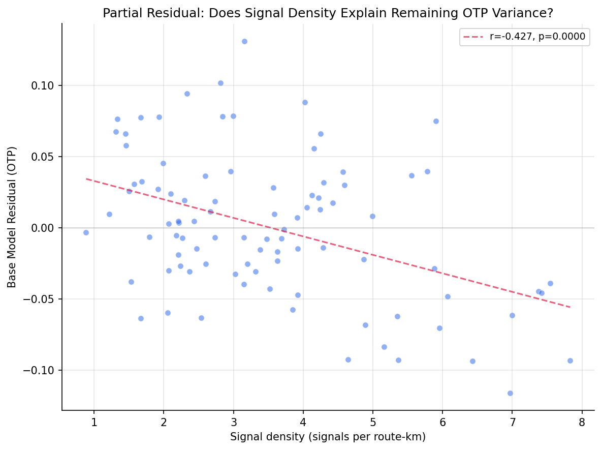
Traffic-signal density is a strong, independent predictor of on-time performance. Routes that pass more traffic signals per mile run measurably later: adding signal density to the six-feature structural model lifts explained OTP variance from 47% to 60% (adjusted R-squared 0.43 to 0.57), and signal density remains highly significant after controlling for stop count, route length, mode, and municipal reach (F-test p < 0.0001). Each additional signal per route-km is associated with roughly 1.75 percentage points lower OTP. This contrasts sharply with Analysis 27, which found that traffic volume (AADT) had no effect — it is the fixed, repeated stop-and-wait of signals, not how busy the road is, that tracks with delay.

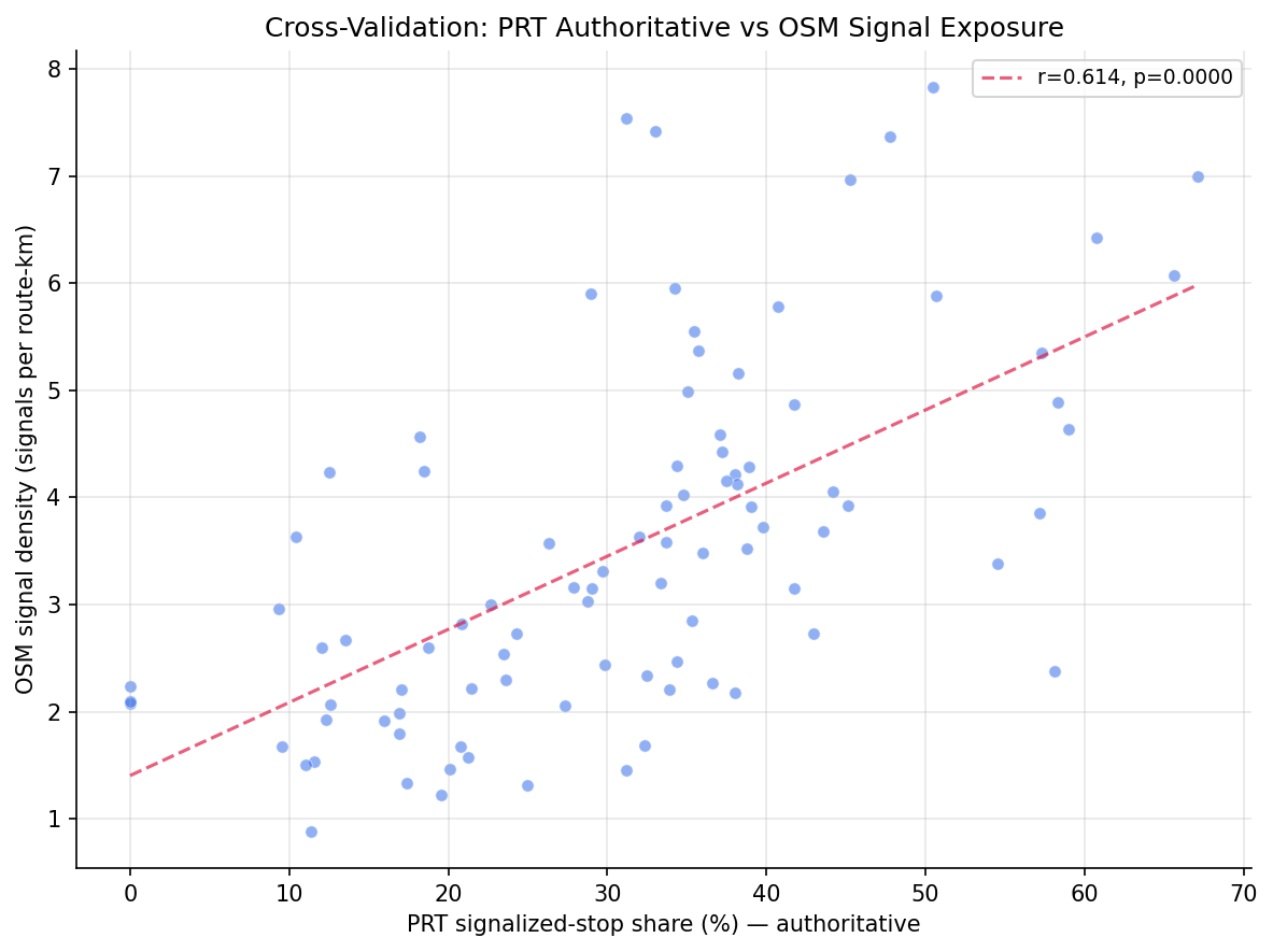
Independently confirmed by PRT's authoritative records. PRT supplied a per-stop signal classification (the stop_signals table). The share of a route's stops that sit at a signal — a completely independent measure of signal exposure — predicts OTP just as strongly (r = −0.50; +13.9 R-squared points beyond the structural model, F = 29.9, p < 0.0001) and agrees with the OpenStreetMap density measure (r = +0.61). When both are entered together they remain significant and non-collinear (VIF ≈ 2.4 each), so the conclusion does not hinge on the crowd-sourced OSM data.

Key Numbers

  • 92 routes analyzed (89 bus, 3 rail) with 12+ months of OTP data and matched signal data.
  • 2,820 OpenStreetMap traffic signals county-wide were matched to GTFS route shapes within a 30 m buffer.
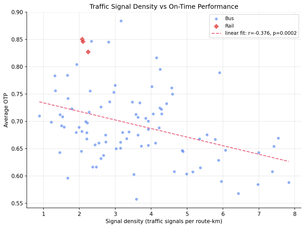
  • Signal density ranges 0.89 to 7.83 signals/km (median ~3.2).
  • Bivariate correlation: signal density vs OTP r = -0.38 (p = 0.0002).
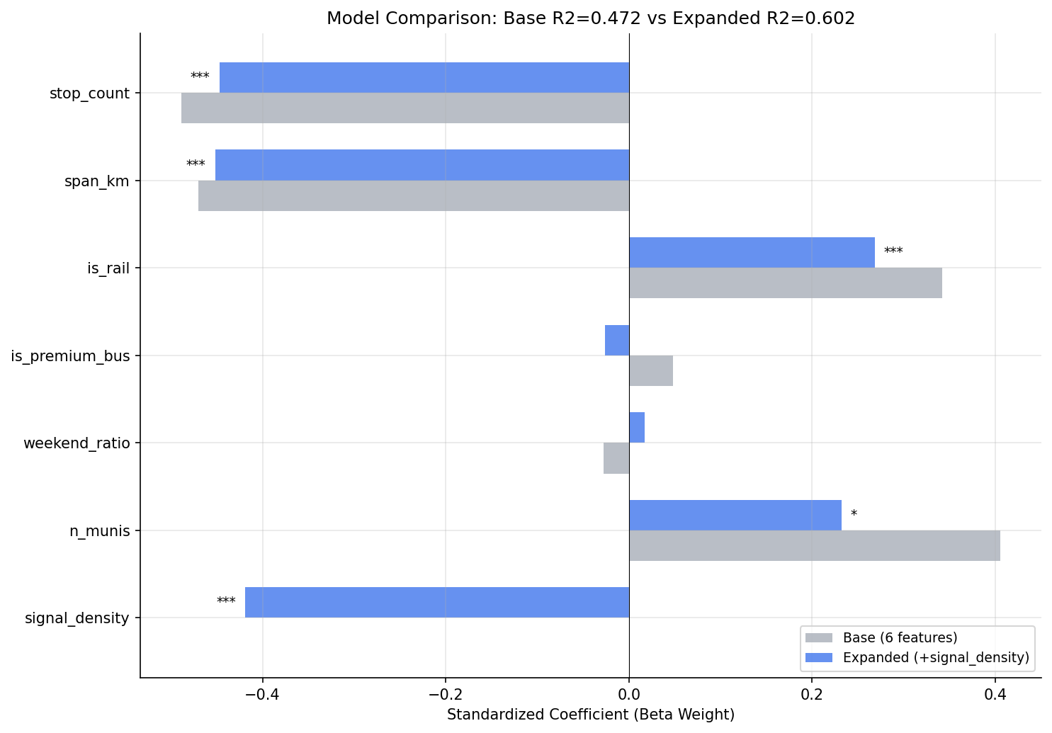
  • Base structural model R-squared 0.472 → expanded model 0.602 (adjusted 0.435 → 0.569); nested F-test p < 0.0001.
  • Expanded-model signal-density coefficient -0.0175 (beta weight -0.42, p < 0.0001) — about -1.75 pp OTP per +1 signal/km.
  • VIF for signal density = 1.35 (all predictors < 5) — no multicollinearity.
  • Bus-only: base R-squared 0.379 → 0.532 (F = 26.9, p < 0.0001, beta -0.45).

Authoritative cross-validation (PRT stop_signals)

  • PRT signalized-stop share vs OSM signal density: r = +0.61 (p < 0.0001); PRT signalized-stop count vs OSM signal count: r = +0.76. The two independent signal-exposure measures agree.
  • PRT signalized-stop share vs OTP: r = −0.50 (p < 0.0001) — the stop-normalized, honest predictor. (Raw count r = −0.70, but it tracks stop_count and is confounded, exactly as raw OSM n_signals is.)
  • Authoritative model (base + sig_stop_share): R-squared 0.472 → 0.611 (+0.139, F = 29.9, p < 0.0001), beta −0.44 — slightly stronger than the OSM density model (+0.130).
  • Combined model (base + density + share): R-squared 0.635; both signal measures stay significant (density p = 0.022, share p = 0.008) with VIF ≈ 2.4 each — distinct, non-redundant facets of signal exposure.

Observations

  • Raw signal count overstates the effect. Raw n_signals correlates with OTP at r = -0.65, but it also correlates with route length at r = +0.47 — a long route passes more signals and tends to run later. Dividing by route length isolates the signal effect: signal density correlates with OTP at the more modest r = -0.38. The regression therefore uses density, not count.
  • Signal density is nearly orthogonal to stop count (r = -0.04). Stops and signals are two separate delay mechanisms — a route can have many stops and few signals, or vice versa — and the model picks up both: in the bus-only expanded model stop count (beta -0.48) and signal density (beta -0.45) are comparably strong, independent predictors.
  • Density still correlates with other geometry (span -0.32, municipal reach -0.39, premium-bus -0.33): suburban and express routes run on faster roads with fewer signals. But the VIF of 1.35 confirms enough independent variation remains for a stable coefficient.
  • The densest-signal routes are inner-city local bus. The top of the list is 71B Highland Park (7.83 signals/km, 59% OTP), 81 Oak Hill, 83 Bedford Hill, 82 Lincoln — all dense East End / Hill District local routes. The sparsest are suburban routes such as 79 East Hills (0.89/km, 71% OTP) and 14 Ohio Valley.
  • Contrast with traffic volume (Analysis 27). AADT had no effect on OTP after structural controls; signal density clearly does. Signals impose a fixed, stochastic delay every cycle regardless of how heavy traffic is, which is a more plausible mechanism for the kind of variance OTP measures.
  • PRT's authoritative records independently confirm the result. The OSM signal exposure was never ground-truthed before. PRT's per-stop classification gives a second, independent measure (what fraction of a route's stops are at a signal); it correlates with the OSM measure (r = +0.61) and predicts OTP just as strongly (r = −0.50, +13.9 R-squared points). The two measures are not redundant (VIF ≈ 2.4 when combined): OSM density counts every signal the route passes (including at non-stop intersections), while the PRT share counts signals where the bus actually stops — two facets of the same delay story.

Discussion

The result reinforces the cumulative picture from Analyses 18, 26 and 27 that OTP is largely a function of route structure. Signal density adds a genuinely new structural axis: it is not captured by stop count (the two are orthogonal) and it explains a meaningful slice of variance the earlier models missed (+13 R-squared points). For policy, the lever is transit-signal priority (TSP) and corridor signal-timing coordination on the dense East End local routes, rather than rerouting — the densest-signal routes are exactly the high-ridership city corridors where rerouting is not an option. The effect is an area-level association, not a trip-level causal estimate; it identifies where signal treatment is most likely to help, not the exact OTP gain a specific TSP project would deliver.

Caveats

  • OpenStreetMap signal coverage is crowd-sourced. The 2,820 county-wide signals fall in the plausible range for Allegheny County (~2,500–3,000), but coverage completeness may vary, likely better in the City of Pittsburgh than in outer suburbs.
  • Density numerator/denominator mismatch. n_signals counts unique signals along the union of all of a route's GTFS shape variants (both directions, all patterns), while length_km is the route's single longest shape. Where the two directions use different parallel streets this modestly inflates density. Most PRT routes run both directions on the same arterials, limiting the effect.
  • Raw signal count is mechanically tied to route length and is reported descriptively only; it is never used as a regression predictor.
  • Ecological framing. All results are route-level associations between signal density and average OTP. No trip-level or rider-level causal claims are made.
  • OLS assumes linear, independent errors. With 92 observations and 7 predictors the model is reasonably but not generously powered.

Validation

  • Data source verified (checklist #1). route_signals is produced by pipeline step 11_signal_overlay; its columns were validated against the ROUTE_SIGNALS schema with validate(..., subset=True). GTFS and OTP columns reuse the same queries as Analysis 27.
  • Scope match (checklist #2). All routes are filtered to 12+ months of OTP and inner-joined to route_signals; signals and routes both cover Allegheny County. 92 of 98 signal-matched routes clear the 12-month OTP threshold.
  • Null handling (checklist #3). signal_density is non-null for every route (all routes have non-zero shape length); drop_nulls guards the structural features. No routes were silently dropped.
  • Aggregate sanity check (checklist #4). Total OSM signal count (2,820) was compared against the known Allegheny County signal inventory order of magnitude (~2,500–3,000) and is consistent. Per-route densities (0.9–7.8/km) imply a signal every 130–1,100 m, plausible for city arterials vs suburban roads.
  • Direction of effect (checklist #6). More signals per km is associated with lower OTP — the expected sign. A positive coefficient would have been a red flag.
  • Multicollinearity checked (checklist #7). VIF is reported for every expanded-model predictor; the maximum is 2.66 and signal density is 1.35. No predictor exceeds the VIF > 5 flag threshold.
  • Small-sample routes flagged (checklist #8). Routes with fewer than 12 months of OTP data are excluded via HAVING COUNT(*) >= 12. The route_signals.match_rate field is not used as a filter — unlike the PennDOT road-network match rate in Analysis 27, it is proportional to signal density and is not a coverage-quality signal.
  • Surprising-result check (checklist #5). The headline (signal density matters where traffic volume did not) was checked for plausibility: signals impose fixed per-cycle delay, a sound mechanism, and the raw-count vs density diagnostic confirmed the relationship is not a route-length artifact.
  • Ecological framing (checklist #9). Documented in Caveats and Discussion; results are described as route-level associations throughout.
  • Cross-validated against an authoritative source (checklist #5). The OSM signal-density measure was checked against PRT's stop_signals records (pipeline 15). The two agree (r = +0.61 share vs density; r = +0.76 counts), and the authoritative measure reproduces the OTP relationship independently. Aggregation joins stop_signalsroute_stops on the PRT internal stop_id (E-code namespace, shared between those two tables); the OSM/GTFS join in Analysis 53 instead keys on stop_code — the two stop-id namespaces differ.

Output
Methods

Methods: Traffic Signals and OTP

Question

Does the density of traffic signals along a route (signals per route-km) explain on-time performance (OTP) variance beyond stop count, geographic span, and the other structural features from the Analysis 18 / 27 model?

Approach

  • Use the route_signals table (built by pipeline step 11_signal_overlay), which counts OpenStreetMap highway=traffic_signals nodes within 30 m of each route's GTFS shape and divides by the route's longest-shape length.
  • Use signal density, not raw signal count, as the predictor. Raw n_signals is mechanically correlated with route length, and route length itself depresses OTP, so a model using raw count would capture a length artifact rather than a signal effect. Raw count is reported descriptively only. As a diagnostic, the bivariate correlations of both n_signals and signal_density against OTP are compared to demonstrate this confound.
  • Replicate the Analysis 27 six-feature OLS base model (stop count, geographic span, is_rail, is_premium_bus, weekend ratio, municipal reach) on routes with matched route_signals data and at least 12 months of OTP observations.
  • Add signal_density as a seventh predictor. Compare adjusted R-squared between the six- and seven-feature models with a nested F-test.
  • Check VIF for multicollinearity. signal_density, stop_count, and span_km all partly encode "urban arterial vs. suburban" route character, so a VIF above 5 is plausible and is reported, not silently dropped.
  • Repeat the comparison on the bus-only subset.
  • The route_signals.match_rate field (fraction of shape points near a signal) is not used as an inclusion filter: unlike the PennDOT road-network match rate in Analysis 27, it is essentially proportional to signal density and is not a coverage-quality signal. It is retained only as a diagnostic column.
  • Cross-validate the OSM signal exposure against PRT's authoritative records. From the stop_signals table (PRT-supplied, pipeline 15_stop_signals), compute each route's sig_stop_share — the fraction of its stops that sit at a traffic signal — and n_sig_stops. Correlate these against the OSM signal_density / n_signals; strong agreement confirms the OSM proxy is sound. As with raw count, sig_stop_share (stop-normalized) is the honest predictor and n_sig_stops is reported only descriptively (it tracks stop count, which itself depresses OTP).
  • Re-test with the authoritative predictor. Fit base + sig_stop_share (Model 3) and base + signal_density + sig_stop_share (Model 4), each with a nested F-test and VIF, to check whether PRT's independent measure confirms the signal→OTP relationship and whether the two signal measures are redundant.
  • Repeat the expanded comparison on the bus-only subset.
  • Generate a bivariate scatter (signal density vs OTP), a coefficient comparison chart, a partial residual plot, and a cross-validation scatter (PRT signalized-stop share vs OSM signal density).

Data

Name Description Source
otp_monthly route_id, month, otp (averaged to route-level, 12+ months required) prt.db table
route_signals route_id, n_signals, length_km, signal_density, match_rate (built by signal_overlay.py) prt.db table
stop_signals per-stop authoritative signal class; aggregated to per-route sig_stop_share / n_sig_stops (built by 15_stop_signals) prt.db table
route_stops stop counts, trip frequencies, stop→route mapping for authoritative aggregation prt.db table
stops lat, lon for geographic span computation; muni for municipal reach prt.db table
routes route_id, mode for subtype classification prt.db table

Output

  • output/model_comparison.csv -- regression results for all models (base, +signal_density, +sig_stop_share, combined, bus-only)
  • output/vif_table.csv -- VIF values for the expanded model
  • output/route_signals_summary.csv -- per-route signal data with OTP, including authoritative n_sig_stops and sig_stop_share
  • output/signal_density_vs_otp_scatter.png -- bivariate scatter of signal density vs OTP
  • output/coefficient_comparison.png -- beta weight comparison between base and expanded models
  • output/partial_residual.png -- partial residual plot for signal density
  • output/cross_validation_signal_exposure.png -- PRT authoritative signalized-stop share vs OSM signal density (proxy validation)

Source Code

"""Analysis 51: Test whether traffic-signal density explains OTP variance beyond structural features."""

import math

import numpy as np
import polars as pl
from scipy import stats

from prt_otp_analysis.common import (
    analysis_dir,
    classify_bus_route,
    correlate,
    phase,
    query_to_polars,
    run_analysis,
    save_chart,
    save_csv,
    setup_plotting,
)
from prt_otp_analysis.common.schemas import ROUTE_SIGNALS, validate

OUT = analysis_dir(__file__)

MIN_MONTHS = 12


# ---------------------------------------------------------------------------
# Helpers (replicated from Analysis 18/27 to maintain independence)
# ---------------------------------------------------------------------------

def haversine_km(lat1: float, lon1: float, lat2: float, lon2: float) -> float:
    """Return the great-circle distance in km between two lat/lon points."""
    R = 6371.0
    dlat = math.radians(lat2 - lat1)
    dlon = math.radians(lon2 - lon1)
    a = (math.sin(dlat / 2) ** 2
         + math.cos(math.radians(lat1)) * math.cos(math.radians(lat2))
         * math.sin(dlon / 2) ** 2)
    return R * 2 * math.atan2(math.sqrt(a), math.sqrt(1 - a))


def compute_span(lats: list[float], lons: list[float]) -> float:
    """Return the max pairwise haversine distance (km) among a set of points."""
    max_dist = 0.0
    n = len(lats)
    for i in range(n):
        for j in range(i + 1, n):
            d = haversine_km(lats[i], lons[i], lats[j], lons[j])
            if d > max_dist:
                max_dist = d
    return max_dist


def compute_vif(X_raw: np.ndarray, feature_names: list[str]) -> dict[str, float]:
    """Compute Variance Inflation Factor for each predictor."""
    n, k = X_raw.shape
    vifs = {}
    for j in range(k):
        y_j = X_raw[:, j]
        X_other = np.delete(X_raw, j, axis=1)
        X_other = np.column_stack([np.ones(n), X_other])
        beta, _, _, _ = np.linalg.lstsq(X_other, y_j, rcond=None)
        y_hat = X_other @ beta
        ss_res = np.sum((y_j - y_hat) ** 2)
        ss_tot = np.sum((y_j - np.mean(y_j)) ** 2)
        r2_j = 1 - ss_res / ss_tot if ss_tot > 0 else 0.0
        vifs[feature_names[j]] = 1.0 / (1.0 - r2_j) if r2_j < 1.0 else float("inf")
    return vifs


def fit_ols(y: np.ndarray, X_raw: np.ndarray, feature_names: list[str]) -> dict:
    """Fit OLS regression and return results dict."""
    n, k = X_raw.shape
    X = np.column_stack([np.ones(n), X_raw])

    beta, _, _, _ = np.linalg.lstsq(X, y, rcond=None)
    y_hat = X @ beta
    residuals = y - y_hat

    ss_res = np.sum(residuals ** 2)
    ss_tot = np.sum((y - np.mean(y)) ** 2)
    r_squared = 1 - ss_res / ss_tot
    adj_r_squared = 1 - (1 - r_squared) * (n - 1) / (n - k - 1)
    mse = ss_res / (n - k - 1)

    XtX_inv = np.linalg.pinv(X.T @ X)
    se = np.sqrt(np.diag(XtX_inv) * mse)
    t_vals = beta / se
    p_vals = [2 * (1 - stats.t.cdf(abs(t), df=n - k - 1)) for t in t_vals]

    x_stds = np.std(X_raw, axis=0, ddof=1)
    y_std = np.std(y, ddof=1)
    beta_weights = beta[1:] * x_stds / y_std

    return {
        "r_squared": r_squared,
        "adj_r_squared": adj_r_squared,
        "ss_res": ss_res,
        "n": n,
        "k": k,
        "features": ["intercept"] + feature_names,
        "coefficients": beta.tolist(),
        "std_errors": se.tolist(),
        "t_values": t_vals.tolist(),
        "p_values": p_vals,
        "beta_weights": [None] + beta_weights.tolist(),
        "y_hat": y_hat,
        "residuals": residuals,
    }


def f_test_nested(base: dict, full: dict) -> tuple[float, float]:
    """F-test comparing nested models. Returns (F_stat, p_value)."""
    k_diff = full["k"] - base["k"]
    n = full["n"]
    f_stat = ((base["ss_res"] - full["ss_res"]) / k_diff) / (full["ss_res"] / (n - full["k"] - 1))
    f_p = 1 - stats.f.cdf(f_stat, k_diff, n - full["k"] - 1)
    return f_stat, f_p


def print_model(results: dict, label: str) -> None:
    """Print formatted model results."""
    print(f"\n  {label}:")
    print(f"  R2 = {results['r_squared']:.4f}, Adj R2 = {results['adj_r_squared']:.4f}, "
          f"n = {results['n']}, k = {results['k']}")
    print(f"  {'Feature':<20s} {'Coeff':>10s} {'Std Err':>10s} {'p-value':>10s} {'Beta':>10s}")
    print(f"  {'-'*60}")
    for i, feat in enumerate(results["features"]):
        coeff = results["coefficients"][i]
        se = results["std_errors"][i]
        p = results["p_values"][i]
        beta = results["beta_weights"][i]
        beta_str = f"{beta:>10.4f}" if beta is not None else f"{'--':>10s}"
        sig = "***" if p < 0.001 else "**" if p < 0.01 else "*" if p < 0.05 else ""
        print(f"  {feat:<20s} {coeff:>10.6f} {se:>10.6f} {p:>10.4f} {beta_str} {sig}")


# ---------------------------------------------------------------------------
# Data loading
# ---------------------------------------------------------------------------

def load_features() -> pl.DataFrame:
    """Assemble structural features + traffic signal data for the regression model."""
    avg_otp = query_to_polars(f"""
        SELECT o.route_id, r.route_name, r.mode,
               AVG(o.otp) AS avg_otp, COUNT(*) AS months
        FROM otp_monthly o
        JOIN routes r ON o.route_id = r.route_id
        GROUP BY o.route_id
        HAVING COUNT(*) >= {MIN_MONTHS}
    """)

    stop_counts = query_to_polars("""
        SELECT route_id, COUNT(DISTINCT stop_id) AS stop_count
        FROM route_stops GROUP BY route_id
    """)
    trips = query_to_polars("""
        SELECT route_id,
               MAX(trips_wd) AS max_wd,
               MAX(trips_sa) AS max_sa,
               MAX(trips_su) AS max_su
        FROM route_stops GROUP BY route_id
    """)
    munis = query_to_polars("""
        SELECT rs.route_id, COUNT(DISTINCT s.muni) AS n_munis
        FROM route_stops rs
        JOIN stops s ON rs.stop_id = s.stop_id
        WHERE s.muni IS NOT NULL AND s.muni != '0'
        GROUP BY rs.route_id
    """)
    stops_by_route = query_to_polars("""
        SELECT rs.route_id, s.lat, s.lon
        FROM route_stops rs
        JOIN stops s ON rs.stop_id = s.stop_id
        WHERE s.lat IS NOT NULL AND s.lon IS NOT NULL
    """)
    spans = []
    for route_id in stops_by_route["route_id"].unique().sort().to_list():
        subset = stops_by_route.filter(pl.col("route_id") == route_id)
        span_km = compute_span(subset["lat"].to_list(), subset["lon"].to_list())
        spans.append({"route_id": route_id, "span_km": span_km})
    span_df = pl.DataFrame(spans)

    # Traffic signal data
    signals_df = query_to_polars("""
        SELECT route_id, n_signals, length_km, signal_density,
               match_rate, n_route_points
        FROM route_signals
    """)
    validate(signals_df, ROUTE_SIGNALS, subset=True)

    # Authoritative per-route signal exposure (PRT stop_signals): how many of a
    # route's stops sit at a traffic signal, and what share. Independent of the
    # OSM density measure above — used to cross-validate it and as an alternative
    # predictor.
    auth_signal_df = query_to_polars("""
        SELECT rs.route_id,
               COUNT(DISTINCT rs.stop_id) AS n_route_stops,
               COUNT(DISTINCT CASE WHEN ss.has_signal = 1 THEN rs.stop_id END)
                   AS n_sig_stops
        FROM route_stops rs
        LEFT JOIN stop_signals ss ON rs.stop_id = ss.stop_id
        GROUP BY rs.route_id
    """).with_columns(
        pl.when(pl.col("n_route_stops") > 0)
        .then(pl.col("n_sig_stops") / pl.col("n_route_stops"))
        .otherwise(None)
        .alias("sig_stop_share"),
    )

    # Assemble
    df = avg_otp
    df = df.join(stop_counts, on="route_id", how="left")
    df = df.join(trips, on="route_id", how="left")
    df = df.join(munis, on="route_id", how="left")
    df = df.join(span_df, on="route_id", how="left")
    df = df.join(signals_df, on="route_id", how="inner")
    df = df.join(auth_signal_df, on="route_id", how="left")

    # Derived features
    df = df.with_columns(
        pl.when(pl.col("max_wd") > 0)
        .then((pl.col("max_sa") + pl.col("max_su")) / (2.0 * pl.col("max_wd")))
        .otherwise(0.0)
        .alias("weekend_ratio"),
    )
    df = df.with_columns(
        pl.when(pl.col("mode") == "RAIL").then(1.0).otherwise(0.0).alias("is_rail"),
    )
    df = df.with_columns(
        pl.when(pl.col("mode") == "BUS")
        .then(pl.col("route_id").map_elements(classify_bus_route, return_dtype=pl.Utf8))
        .otherwise(pl.lit("non_bus"))
        .alias("bus_subtype"),
    )
    df = df.with_columns(
        pl.when(pl.col("bus_subtype").is_in(["busway", "flyer", "express", "limited"]))
        .then(1.0)
        .otherwise(0.0)
        .alias("is_premium_bus"),
    )

    df = df.drop_nulls(
        subset=["stop_count", "span_km", "weekend_ratio", "n_munis",
                "signal_density", "sig_stop_share"],
    )

    return df


# ---------------------------------------------------------------------------
# Charts
# ---------------------------------------------------------------------------

def make_scatter_chart(df: pl.DataFrame) -> None:
    """Bivariate scatter: signal density vs OTP."""
    plt = setup_plotting()
    fig, ax = plt.subplots(figsize=(8, 6))

    density = df["signal_density"].to_numpy()
    otp = df["avg_otp"].to_numpy()
    modes = df["mode"].to_list()

    bus_mask = np.array([m == "BUS" for m in modes])
    rail_mask = ~bus_mask

    ax.scatter(density[bus_mask], otp[bus_mask], alpha=0.5, s=30, color="#2563eb",
               edgecolors="white", linewidth=0.5, label="Bus", zorder=2)
    if np.any(rail_mask):
        ax.scatter(density[rail_mask], otp[rail_mask], alpha=0.7, s=50, color="#dc2626",
                   marker="D", edgecolors="white", linewidth=0.5, label="Rail", zorder=3)

    # Trend line (all routes)
    slope, intercept, r, p, _ = stats.linregress(density, otp)
    x_sorted = np.sort(density)
    ax.plot(x_sorted, slope * x_sorted + intercept, color="#e11d48",
            linewidth=1.5, linestyle="--", alpha=0.7,
            label=f"linear fit: r={r:.3f}, p={p:.4f}")

    ax.set_xlabel("Signal density (traffic signals per route-km)")
    ax.set_ylabel("Average OTP")
    ax.set_title("Traffic Signal Density vs On-Time Performance")
    ax.legend(fontsize=9)

    save_chart(fig, OUT / "signal_density_vs_otp_scatter.png")


def make_coefficient_chart(base: dict, expanded: dict) -> None:
    """Compare standardized coefficients between base and expanded models."""
    plt = setup_plotting()
    fig, ax = plt.subplots(figsize=(10, 7))

    base_feats = base["features"][1:]
    exp_feats = expanded["features"][1:]
    base_betas = {f: b for f, b in zip(base_feats, base["beta_weights"][1:])}
    exp_betas = {f: b for f, b in zip(exp_feats, expanded["beta_weights"][1:])}
    exp_pvals = {f: p for f, p in zip(exp_feats, expanded["p_values"][1:])}

    all_feats = exp_feats
    y_pos = np.arange(len(all_feats))
    width = 0.35

    base_vals = [base_betas.get(f, 0.0) for f in all_feats]
    exp_vals = [exp_betas[f] for f in all_feats]

    ax.barh(y_pos + width / 2, base_vals, width, label="Base (6 features)",
            color="#9ca3af", alpha=0.7)
    ax.barh(y_pos - width / 2, exp_vals, width, label="Expanded (+signal_density)",
            color="#2563eb", alpha=0.7)

    for i, f in enumerate(all_feats):
        p = exp_pvals[f]
        marker = "***" if p < 0.001 else "**" if p < 0.01 else "*" if p < 0.05 else ""
        val = exp_vals[i]
        ax.text(val + 0.01 if val >= 0 else val - 0.01, i - width / 2, marker,
                ha="left" if val >= 0 else "right", va="center", fontsize=9)

    ax.set_yticks(y_pos)
    ax.set_yticklabels(all_feats)
    ax.axvline(0, color="black", linewidth=0.5)
    ax.set_xlabel("Standardized Coefficient (Beta Weight)")
    ax.set_title(f"Model Comparison: Base R2={base['r_squared']:.3f} vs "
                 f"Expanded R2={expanded['r_squared']:.3f}")
    ax.legend(loc="lower right", fontsize=9)
    ax.invert_yaxis()

    save_chart(fig, OUT / "coefficient_comparison.png")


def make_partial_residual_chart(df: pl.DataFrame, base: dict) -> None:
    """Partial residual plot: base model residuals vs signal density."""
    plt = setup_plotting()
    fig, ax = plt.subplots(figsize=(8, 6))

    residuals = base["residuals"]
    density = df["signal_density"].to_numpy()

    ax.scatter(density, residuals, alpha=0.5, s=30, color="#2563eb",
               edgecolors="white", linewidth=0.5)

    slope, intercept, r, p, _ = stats.linregress(density, residuals)
    x_line = np.array([density.min(), density.max()])
    ax.plot(x_line, slope * x_line + intercept, color="#e11d48", linewidth=1.5,
            linestyle="--", alpha=0.7, label=f"r={r:.3f}, p={p:.4f}")

    ax.axhline(0, color="gray", linewidth=0.5, alpha=0.5)
    ax.set_xlabel("Signal density (signals per route-km)")
    ax.set_ylabel("Base Model Residual (OTP)")
    ax.set_title("Partial Residual: Does Signal Density Explain Remaining OTP Variance?")
    ax.legend(fontsize=9)

    save_chart(fig, OUT / "partial_residual.png")


def make_cross_validation_chart(df: pl.DataFrame) -> None:
    """Scatter: PRT authoritative signalized-stop share vs OSM signal density."""
    plt = setup_plotting()
    fig, ax = plt.subplots(figsize=(8, 6))

    share = df["sig_stop_share"].to_numpy() * 100
    density = df["signal_density"].to_numpy()

    ax.scatter(share, density, alpha=0.5, s=30, color="#2563eb",
               edgecolors="white", linewidth=0.5)
    slope, intercept, r, p, _ = stats.linregress(share, density)
    x_line = np.array([share.min(), share.max()])
    ax.plot(x_line, slope * x_line + intercept, color="#e11d48", linewidth=1.5,
            linestyle="--", alpha=0.7, label=f"r={r:.3f}, p={p:.4f}")

    ax.set_xlabel("PRT signalized-stop share (%) — authoritative")
    ax.set_ylabel("OSM signal density (signals per route-km)")
    ax.set_title("Cross-Validation: PRT Authoritative vs OSM Signal Exposure")
    ax.legend(fontsize=9)

    save_chart(fig, OUT / "cross_validation_signal_exposure.png")


# ---------------------------------------------------------------------------
# Main
# ---------------------------------------------------------------------------

@run_analysis(51, "Traffic Signals and OTP")
def main() -> None:
    """Entry point: load features, fit models, compare, chart, and save."""

    with phase("Loading and assembling features"):
        df = load_features()
        n_rail = len(df.filter(pl.col("is_rail") == 1.0))
        n_bus = len(df.filter(pl.col("mode") == "BUS"))
        print(f"  {len(df)} routes with signal + structural features "
              f"({n_bus} BUS, {n_rail} RAIL)")
        print(f"  Signal density range: {df['signal_density'].min():.2f} -- "
              f"{df['signal_density'].max():.2f} signals/km")
        print(f"  Signal count range: {df['n_signals'].min()} -- {df['n_signals'].max()}")
        print(f"  Median match rate (diagnostic only): {df['match_rate'].median():.1%}")

    y = df["avg_otp"].to_numpy()

    # --- Diagnostic: raw count vs density bivariate correlations ---
    with phase("Diagnostic: raw count vs density confound"):
        corr_count = correlate(df, "n_signals", "avg_otp")
        corr_density = correlate(df, "signal_density", "avg_otp")
        corr_count_len = correlate(df, "n_signals", "length_km")
        print(f"  n_signals      vs avg_otp : r = {corr_count['pearson_r']:+.3f}, "
              f"p = {corr_count['pearson_p']:.4f}")
        print(f"  signal_density vs avg_otp : r = {corr_density['pearson_r']:+.3f}, "
              f"p = {corr_density['pearson_p']:.4f}")
        print(f"  n_signals      vs length  : r = {corr_count_len['pearson_r']:+.3f}, "
              f"p = {corr_count_len['pearson_p']:.4f}")
        print("  => raw n_signals tracks route length; signal_density is the "
              "length-adjusted predictor.")

    # --- Cross-validation: OSM signal exposure vs PRT authoritative ---
    with phase("Cross-validating OSM signals against PRT authoritative stops"):
        cv_density = correlate(df, "sig_stop_share", "signal_density")
        cv_count = correlate(df, "n_sig_stops", "n_signals")
        share_otp = correlate(df, "sig_stop_share", "avg_otp")
        nsig_otp = correlate(df, "n_sig_stops", "avg_otp")
        print(f"  PRT sig_stop_share vs OSM signal_density : r = {cv_density['pearson_r']:+.3f}, "
              f"p = {cv_density['pearson_p']:.4f}")
        print(f"  PRT n_sig_stops    vs OSM n_signals      : r = {cv_count['pearson_r']:+.3f}, "
              f"p = {cv_count['pearson_p']:.4f}")
        print("  => the two independent signal-exposure measures agree, validating "
              "the OSM proxy used in the headline model.")
        print(f"  PRT sig_stop_share vs avg_otp : r = {share_otp['pearson_r']:+.3f}, "
              f"p = {share_otp['pearson_p']:.4f}  (length-adjusted, honest predictor)")
        print(f"  PRT n_sig_stops    vs avg_otp : r = {nsig_otp['pearson_r']:+.3f}, "
              f"p = {nsig_otp['pearson_p']:.4f}  (tracks stop_count — confounded)")

    # --- Model 1: Base (Analysis 27 replication, 6 features) ---
    base_features = ["stop_count", "span_km", "is_rail", "is_premium_bus",
                     "weekend_ratio", "n_munis"]
    X_base = np.column_stack([df[f].to_numpy().astype(float) for f in base_features])
    with phase("Fitting base model (6 features, Analysis 27 replication)"):
        base = fit_ols(y, X_base, base_features)
        print_model(base, "Base model (6 features)")

    # --- Model 2: Expanded (+ signal_density) ---
    exp_features = base_features + ["signal_density"]
    X_exp = np.column_stack([df[f].to_numpy().astype(float) for f in exp_features])
    with phase("Fitting expanded model (+ signal_density)"):
        expanded = fit_ols(y, X_exp, exp_features)
        print_model(expanded, "Expanded model (+ signal_density)")

        f_stat, f_p = f_test_nested(base, expanded)
        print(f"\n  F-test for signal_density: F = {f_stat:.3f}, p = {f_p:.4f}")
        print(f"  R2 change: {base['r_squared']:.4f} -> {expanded['r_squared']:.4f} "
              f"(+{expanded['r_squared'] - base['r_squared']:.4f})")
        print(f"  Adj R2 change: {base['adj_r_squared']:.4f} -> {expanded['adj_r_squared']:.4f} "
              f"({expanded['adj_r_squared'] - base['adj_r_squared']:+.4f})")
        if f_p < 0.05:
            print("  => signal density IS significant after controlling for "
                  "structural features.")
        else:
            print("  => signal density is NOT significant after controlling for "
                  "structural features.")

        # --- VIF for expanded model ---
        print("\n--- VIF (Expanded Model: base + signal_density) ---")
        vifs = compute_vif(X_exp, exp_features)
        for feat, vif in vifs.items():
            flag = " ** HIGH" if vif > 5 else ""
            print(f"  {feat:<20s} VIF = {vif:.2f}{flag}")

        # --- Correlation: signal_density vs structural features ---
        print("\n--- Correlations: signal_density vs structural features ---")
        for feat in base_features:
            corr = correlate(df, feat, "signal_density")
            sig = "*" if corr["pearson_p"] < 0.05 else ""
            print(f"  signal_density vs {feat:<16s}: r = {corr['pearson_r']:+.3f}, "
                  f"p = {corr['pearson_p']:.4f} {sig}")

    # --- Model 3: Authoritative (base + PRT signalized-stop share) ---
    auth_features = base_features + ["sig_stop_share"]
    X_auth = np.column_stack([df[f].to_numpy().astype(float) for f in auth_features])
    with phase("Fitting authoritative model (+ PRT sig_stop_share)"):
        auth_model = fit_ols(y, X_auth, auth_features)
        print_model(auth_model, "Authoritative model (+ sig_stop_share)")
        f_auth, fp_auth = f_test_nested(base, auth_model)
        print(f"\n  F-test for sig_stop_share: F = {f_auth:.3f}, p = {fp_auth:.4f}")
        print(f"  R2 change: {base['r_squared']:.4f} -> {auth_model['r_squared']:.4f} "
              f"(+{auth_model['r_squared'] - base['r_squared']:.4f})")
        if fp_auth < 0.05:
            print("  => PRT authoritative signal exposure IS significant beyond "
                  "structural features — independently confirms the OSM result.")

    # --- Model 4: Combined (base + OSM density + PRT share) ---
    combined_features = base_features + ["signal_density", "sig_stop_share"]
    X_comb = np.column_stack([df[f].to_numpy().astype(float) for f in combined_features])
    with phase("Fitting combined model (+ signal_density + sig_stop_share)"):
        combined = fit_ols(y, X_comb, combined_features)
        print_model(combined, "Combined model (density + share)")
        f_comb, fp_comb = f_test_nested(base, combined)
        print(f"\n  F-test (both signal measures): F = {f_comb:.3f}, p = {fp_comb:.4f}")
        print(f"  R2: base {base['r_squared']:.4f} -> combined {combined['r_squared']:.4f}")
        comb_vifs = compute_vif(X_comb, combined_features)
        print("  VIF (density, share): "
              f"{comb_vifs['signal_density']:.2f}, {comb_vifs['sig_stop_share']:.2f}")
        dens_p = combined["p_values"][combined_features.index("signal_density") + 1]
        share_p = combined["p_values"][combined_features.index("sig_stop_share") + 1]
        if dens_p < 0.05 and share_p < 0.05:
            print("  => both remain significant and non-collinear: signal density "
                  "and signalized-stop share capture distinct delay facets.")

    # --- Bus-only subgroup ---
    bus_df = df.filter(pl.col("mode") == "BUS")
    y_bus = bus_df["avg_otp"].to_numpy()
    bus_base_feats = ["stop_count", "span_km", "is_premium_bus", "weekend_ratio", "n_munis"]
    bus_exp_feats = bus_base_feats + ["signal_density"]

    X_bus_base = np.column_stack([bus_df[f].to_numpy().astype(float) for f in bus_base_feats])
    X_bus_exp = np.column_stack([bus_df[f].to_numpy().astype(float) for f in bus_exp_feats])

    with phase(f"Fitting bus-only models ({len(bus_df)} routes)"):
        bus_base = fit_ols(y_bus, X_bus_base, bus_base_feats)
        print_model(bus_base, "Bus-only base (5 features)")

        bus_expanded = fit_ols(y_bus, X_bus_exp, bus_exp_feats)
        print_model(bus_expanded, "Bus-only expanded (+ signal_density)")

        f_bus, fp_bus = f_test_nested(bus_base, bus_expanded)
        print(f"\n  Bus-only F-test for signal_density: F = {f_bus:.3f}, p = {fp_bus:.4f}")
        print(f"  R2 change: {bus_base['r_squared']:.4f} -> {bus_expanded['r_squared']:.4f} "
              f"(+{bus_expanded['r_squared'] - bus_base['r_squared']:.4f})")

    with phase("Saving CSVs"):
        rows = []
        models = [
            (base, "base_6feat"),
            (expanded, "expanded_7feat_signal_density"),
            (auth_model, "authoritative_sig_stop_share"),
            (combined, "combined_density_and_share"),
            (bus_base, "bus_base"),
            (bus_expanded, "bus_expanded_signal_density"),
        ]
        for model, label in models:
            for i, feat in enumerate(model["features"]):
                rows.append({
                    "model": label,
                    "feature": feat,
                    "coefficient": model["coefficients"][i],
                    "std_error": model["std_errors"][i],
                    "p_value": model["p_values"][i],
                    "beta_weight": model["beta_weights"][i]
                    if model["beta_weights"][i] is not None else float("nan"),
                    "r_squared": model["r_squared"],
                    "adj_r_squared": model["adj_r_squared"],
                    "n": model["n"],
                })
        save_csv(pl.DataFrame(rows), OUT / "model_comparison.csv")

        vif_df = pl.DataFrame([{"feature": f, "vif": v} for f, v in vifs.items()])
        save_csv(vif_df, OUT / "vif_table.csv")

        summary_df = df.select([
            "route_id", "route_name", "mode", "avg_otp", "n_signals",
            "length_km", "signal_density", "match_rate", "stop_count", "span_km",
            "n_route_stops", "n_sig_stops", "sig_stop_share",
        ]).sort("signal_density", descending=True)
        save_csv(summary_df, OUT / "route_signals_summary.csv")

    with phase("Generating charts"):
        make_scatter_chart(df)
        make_coefficient_chart(base, expanded)
        make_partial_residual_chart(df, base)
        make_cross_validation_chart(df)


if __name__ == "__main__":
    main()

Sources

NameTypeWhy It MattersOwnerFreshnessCaveat
otp_monthly table Primary analytical table used in this page's computations. Produced by Data Ingestion. Updated when the producing pipeline step is rerun. Coverage depends on upstream source availability and ETL assumptions.
Upstream sources (5)
  • file data/routes_by_month.csv — Monthly route OTP source table in wide format.
  • file data/PRT_Current_Routes_Full_System_de0e48fcbed24ebc8b0d933e47b56682.csv — Current route metadata and mode classifications.
  • file data/Transit_stops_(current)_by_route_e040ee029227468ebf9d217402a82fa9.csv — Current stop-to-route coverage and trip counts.
  • file data/PRT_Stop_Reference_Lookup_Table.csv — Historical stop reference file with geography attributes.
  • file data/average-ridership/12bb84ed-397e-435c-8d1b-8ce543108698.csv — Average ridership by route and month.
route_signals table Primary analytical table used in this page's computations. Produced by Signal Overlay ETL. Updated when the producing pipeline step is rerun. Coverage depends on upstream source availability and ETL assumptions.
Upstream sources (4)
  • file data/osm-signals/traffic_signals_raw.json — Cached OpenStreetMap Overpass response of traffic-signal nodes for Allegheny County.
  • file data/GTFS/shapes.txt — GTFS route shape geometry points.
  • file data/GTFS/trips.txt — GTFS shape-to-route mapping.
  • api OpenStreetMap Overpass API — Public query endpoint for OSM nodes tagged highway=traffic_signals.
stop_signals table Primary analytical table used in this page's computations. Produced by PRT Stop-Signal Classification ETL. Updated when the producing pipeline step is rerun. Coverage depends on upstream source availability and ETL assumptions.
Upstream sources (1)
  • file data/prt-stop-signals/bus_stops_with_signals_2602.xlsx — PRT-provided spreadsheet (Samuel Buckley, 2026) tagging each of 6,306 bus stops as no-signal, near-side, far-side, or busway/BRT.
route_stops table Primary analytical table used in this page's computations. Produced by Data Ingestion. Updated when the producing pipeline step is rerun. Coverage depends on upstream source availability and ETL assumptions.
Upstream sources (5)
  • file data/routes_by_month.csv — Monthly route OTP source table in wide format.
  • file data/PRT_Current_Routes_Full_System_de0e48fcbed24ebc8b0d933e47b56682.csv — Current route metadata and mode classifications.
  • file data/Transit_stops_(current)_by_route_e040ee029227468ebf9d217402a82fa9.csv — Current stop-to-route coverage and trip counts.
  • file data/PRT_Stop_Reference_Lookup_Table.csv — Historical stop reference file with geography attributes.
  • file data/average-ridership/12bb84ed-397e-435c-8d1b-8ce543108698.csv — Average ridership by route and month.
routes table Primary analytical table used in this page's computations. Produced by Data Ingestion. Updated when the producing pipeline step is rerun. Coverage depends on upstream source availability and ETL assumptions.
Upstream sources (5)
  • file data/routes_by_month.csv — Monthly route OTP source table in wide format.
  • file data/PRT_Current_Routes_Full_System_de0e48fcbed24ebc8b0d933e47b56682.csv — Current route metadata and mode classifications.
  • file data/Transit_stops_(current)_by_route_e040ee029227468ebf9d217402a82fa9.csv — Current stop-to-route coverage and trip counts.
  • file data/PRT_Stop_Reference_Lookup_Table.csv — Historical stop reference file with geography attributes.
  • file data/average-ridership/12bb84ed-397e-435c-8d1b-8ce543108698.csv — Average ridership by route and month.
stops table Primary analytical table used in this page's computations. Produced by Data Ingestion. Updated when the producing pipeline step is rerun. Coverage depends on upstream source availability and ETL assumptions.
Upstream sources (5)
  • file data/routes_by_month.csv — Monthly route OTP source table in wide format.
  • file data/PRT_Current_Routes_Full_System_de0e48fcbed24ebc8b0d933e47b56682.csv — Current route metadata and mode classifications.
  • file data/Transit_stops_(current)_by_route_e040ee029227468ebf9d217402a82fa9.csv — Current stop-to-route coverage and trip counts.
  • file data/PRT_Stop_Reference_Lookup_Table.csv — Historical stop reference file with geography attributes.
  • file data/average-ridership/12bb84ed-397e-435c-8d1b-8ce543108698.csv — Average ridership by route and month.
numpy dependency Runtime dependency required for this page's pipeline or analysis code. Open-source Python ecosystem maintainers. Version pinned by project environment until dependency updates are applied. Library updates may change behavior or defaults.
polars dependency Runtime dependency required for this page's pipeline or analysis code. Open-source Python ecosystem maintainers. Version pinned by project environment until dependency updates are applied. Library updates may change behavior or defaults.
scipy dependency Runtime dependency required for this page's pipeline or analysis code. Open-source Python ecosystem maintainers. Version pinned by project environment until dependency updates are applied. Library updates may change behavior or defaults.