Analysis

48 - Service Productivity (Passengers per Revenue Hour)

Equity and Strategic Planning

Coverage: Coverage window unavailable for this page.

Built 2026-06-15 11:52 UTC · Commit e5cf673

Page Navigation

Analysis Navigation

Data Provenance

flowchart LR
  48_service_productivity(["48 - Service Productivity (Passengers per Revenue Hour)"])
  t_ntd_annual_service[("ntd_annual_service")] --> 48_service_productivity
  06_ntd_service[["NTD Annual Service ETL"]] --> t_ntd_annual_service
  u1_06_ntd_service[/"data/ntd-annual-service/2023_TS2.2_Service_Data.xlsx"/] --> 06_ntd_service
  d1_48_service_productivity(("polars (lib)")) --> 48_service_productivity
  d2_48_service_productivity(("matplotlib (lib)")) --> 48_service_productivity
  classDef page fill:#dbeafe,stroke:#1d4ed8,color:#1e3a8a,stroke-width:2px;
  classDef table fill:#ecfeff,stroke:#0e7490,color:#164e63;
  classDef dep fill:#fff7ed,stroke:#c2410c,color:#7c2d12,stroke-dasharray: 4 2;
  classDef file fill:#eef2ff,stroke:#6366f1,color:#3730a3;
  classDef api fill:#f0fdf4,stroke:#16a34a,color:#14532d;
  classDef pipeline fill:#f5f3ff,stroke:#7c3aed,color:#4c1d95;
  class 48_service_productivity page;
  class t_ntd_annual_service table;
  class d1_48_service_productivity,d2_48_service_productivity dep;
  class u1_06_ntd_service file;
  class 06_ntd_service pipeline;

Findings

Findings: Service Productivity (Passengers per Revenue Hour)

Key findings

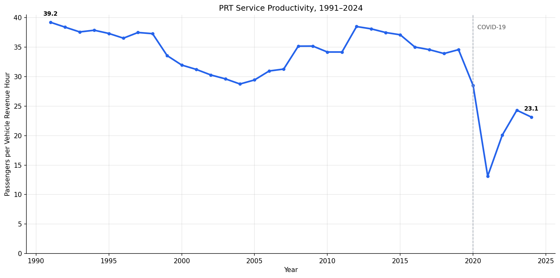
  1. PRT's fixed-route service productivity fell 41% since 1991 — from 39.2 passengers per vehicle revenue hour in 1991 to 23.1 in 2024. Each hour of bus and rail service now carries about two-thirds as many riders as it did three decades ago. (Note: the agency-wide figure including ACCESS paratransit is 18.3 in 2024; see Limitations.)

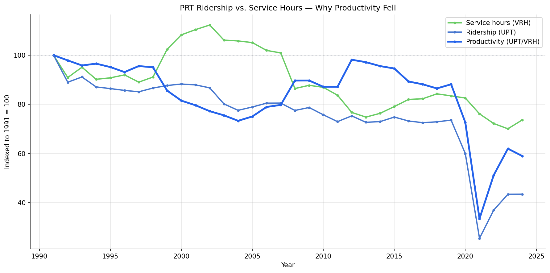
  2. Both service and ridership fell, but ridership fell faster. Over the full 1991–2024 record, PRT's fixed-route service hours dropped 26% (VRH −26%) while fixed-route ridership collapsed 57% (UPT −57%). PRT has cut substantial service — the collapse is not a story of service holding steady while riders vanished — but it couldn't cut fast enough to match the pace of ridership loss.

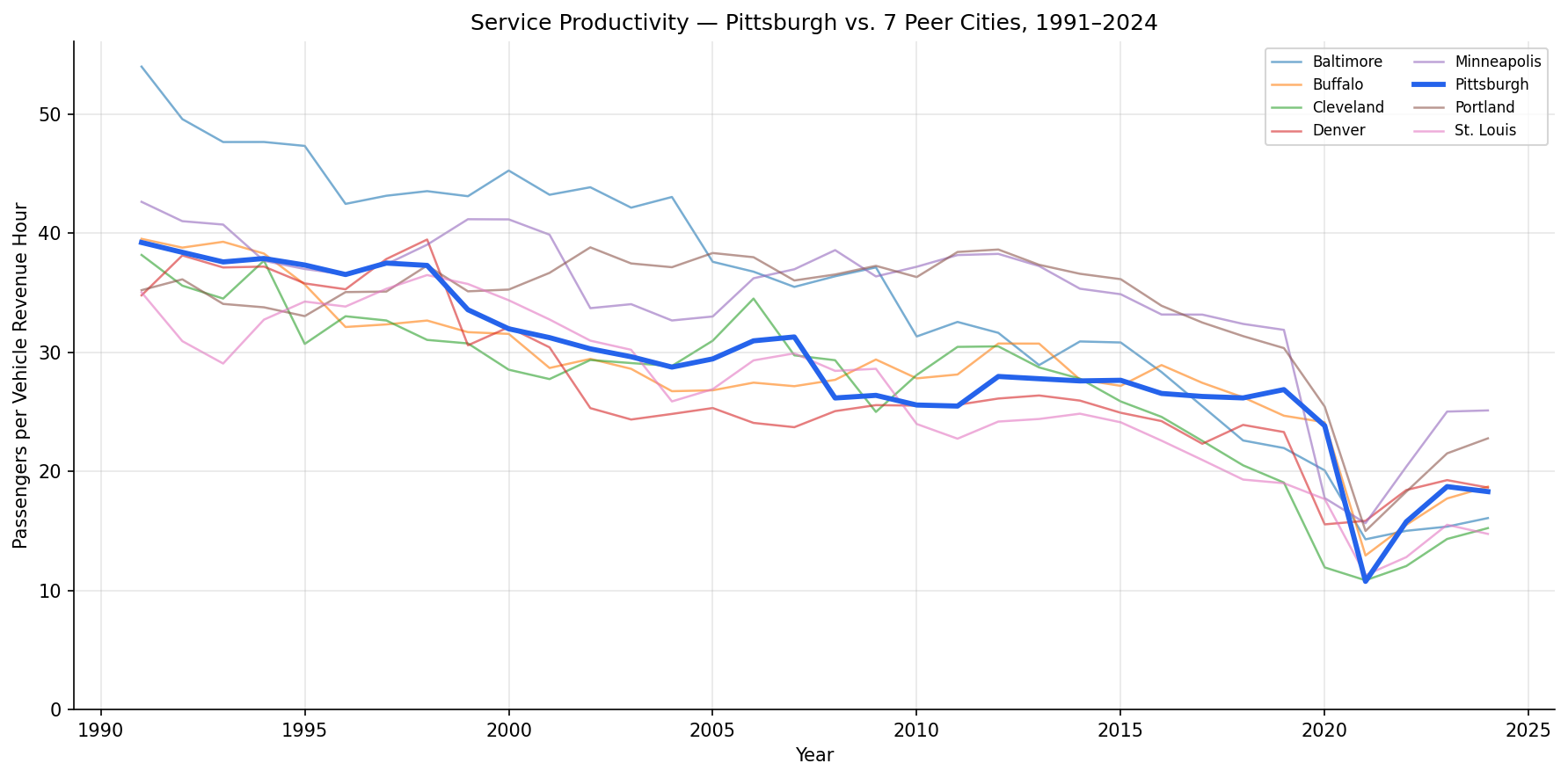
  3. PRT's post-pandemic productivity drop was the steepest of all 8 peer cities. Between 2019 and 2024, PRT agency-wide productivity fell 32% (26.9 → 18.3), worse than every peer — Portland (−25%), Baltimore (−27%), Buffalo (−24%), St. Louis (−22%), Minneapolis (−21%), Cleveland (−20%), Denver (−20%).

  4. The decline is long-run, not just a COVID shock. PRT agency-wide productivity had already fallen 31% from 1991 (39.2) to 2019 (26.9) before the pandemic. COVID then roughly doubled the cumulative loss in five years.

  5. PRT's 2024 agency-wide productivity (18.3) is mid-pack, leaning low. It trails Minneapolis (25.1), Portland (22.8), Buffalo (18.7), and Denver (18.6), and sits above Baltimore (16.1), Cleveland (15.2), and St. Louis (14.7). Productivity fell at every peer — this is a national pattern, not a Pittsburgh-specific failure — but Pittsburgh's rate of recent decline stands out.

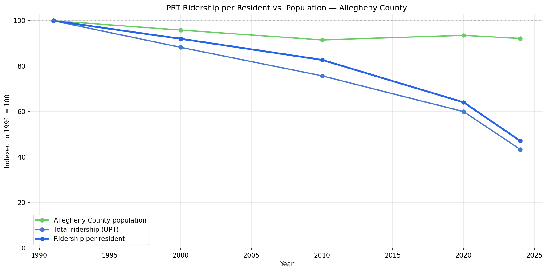
  6. Population decline explains only about a tenth of the drop. PRT serves Allegheny County, which lost roughly 8% of its residents between the 1990 census (1,336,449) and 2024 (1,231,809). But fixed-route ridership fell 57% over the same span, so ridership per resident roughly halved — from 63.7 to 30.0 trips per resident per year. A log decomposition of the ridership decline attributes ~10% to fewer residents and ~90% to each remaining resident riding less. Because service hours also fell, the same split applies to the productivity decline: depopulation is a minor factor, and the collapse is overwhelmingly a demand problem.

Limitations

  • Two metrics in use. Findings 1-2 and the per-capita analysis use a corrected fixed-route VRH series for PRT (see Data Quality note below). Findings 3-5 and the peer comparison charts use the NTD annual workbook (ntd_annual_service), which aggregates all modes — mixing motor bus, light rail, the ACCESS paratransit service, and the incline — and is the only consistently available source for all 8 agencies across the full period.
  • ACCESS paratransit VRH reporting discontinuity. ntd_annual_service excluded ACCESS (demand-response / DR mode) VRH before 2008, then started including ~700K hours/year. This creates an artificial 18% jump in the aggregate VRH for 2008 that does not reflect real service expansion. The PRT trend and decomposition charts correct for this by subtracting DR VRH (and UPT) for 2008 onward using mode-level data from ntd_ridership. The peer comparison charts use the uncorrected agency-wide aggregate, which is internally consistent across agencies for comparison purposes.
  • UPT counts boardings, not riders. Unlinked passenger trips count each boarding separately, so a rider who transfers is counted more than once. Productivity here measures boardings per service hour, not unique people moved.
  • VRH excludes deadhead. Vehicle revenue hours count only time in revenue service, not pull-out, layover, or repositioning, so this understates total operating effort behind each productive hour.
  • Productivity is not the only goal. Lower productivity can reflect a deliberate equity choice to serve lower-density areas. The metric describes how full the service runs, not whether the service is worth running.
  • Population normalization is coarse. County population is paired with the NTD record only at census/estimate years (1990/2000/2010/2020 decennial counts plus the 2024 estimate), with no annual interpolation; the 1990 count stands in for 1991 with a ~9-month offset. Allegheny County is also broader than PRT's true ridership catchment, so the per-capita figures are county-wide averages, not the usage of the population actually within reach of service. The ~10% population share is approximate but robust — even the City of Pittsburgh's steeper ~18% loss would still leave per-capita decline as the dominant factor.

Validation

  • Data source verified. upt and vrh columns of ntd_annual_service (NTD annual data, TS2.2). Mode-level correction uses ntd_ridership (NTD monthly data). No column mapping written from memory. Allegheny County population is from the U.S. Census Bureau: decennial counts for 1990–2020 and the Vintage 2024 Population Estimates Program figure.
  • ACCESS correction verified. For 2007, ntd_annual_service VRH (2,190,548) matches ntd_ridership MB+LR+IP sum (~2,093K) — confirming ACCESS was not in the aggregate. For 2008, ntd_annual_service VRH (2,587,521) matches MB+LR+IP+DR combined (~2,609K) — confirming ACCESS was added. The corrected 2008 fixed-route VRH (1,876,019) is consistent with the documented June 2007 Port Authority service cuts.
  • Population discontinuity avoided. Decennial census counts and intercensal estimates use different methods; mixing a pre-2020 estimate with the 2020 census produces a spurious population jump. The decomposition uses only decennial counts plus one post-2020 estimate, so no method break falls inside the series.
  • Null/missing handling. All 8 peer agencies have complete, non-null UPT and VRH for every year 1991–2024 (34 city-years each) — verified before analysis. No rows dropped.
  • Aggregates sanity-checked. PRT 2024 agency-wide UPT (37.9M) and VRH (2.07M) match the figures used in Analysis 40. The corrected fixed-route 2024 values (UPT 37.0M, VRH 1.60M) are consistent with Analysis 50's mode-level breakdown.
  • Direction of effects checked. Productivity fell at all 8 agencies post-COVID, consistent with the well-documented national decline in transit ridership relative to service. No directional reversal. The corrected VRH series confirms fixed-route service WAS cut substantially (−26%) and the service cuts are consistent with published news reports of Port Authority cutbacks in 2007 and subsequent years.
  • Surprising result investigated. The original (uncorrected) chart showed VRH rising in 2007-08 despite documented service cuts. Investigation confirmed this was an NTD reporting change (ACCESS added to aggregate in 2008), not real service expansion. The corrected series shows fixed-route VRH declining from 2008 onward, consistent with reported service cuts.

Output
Methods

Methods: Service Productivity (Passengers per Revenue Hour)

Question

Has PRT's service productivity — the number of passengers carried per hour of service operated — declined over time? And if so, is the decline because ridership fell faster than service was cut (emptier buses) rather than a deliberate right-sizing of service to match demand?

Approach

  • Define service productivity as unlinked passenger trips per vehicle revenue hour: productivity = UPT / VRH. This is the standard transit efficiency ratio — how many riders each hour of operated service actually carried.
  • Pull the full 1991–2024 annual record of UPT and VRH for PRT and 7 peer cities from ntd_annual_service.
  • For PRT trend and decomposition charts, build a corrected fixed-route series to remove an NTD reporting discontinuity: ntd_annual_service excluded ACCESS paratransit (DR mode) from VRH before 2008, then started including ~700K hours/year. For years ≥ 2008, DR UPT and VRH are subtracted from the aggregate using annual sums from ntd_ridership. Peer comparison charts continue to use ntd_annual_service directly (consistent across all 8 agencies).
  • Plot PRT's productivity curve across the whole record to separate the long-run secular trend from the COVID shock.
  • Decompose the ratio: index UPT, VRH, and productivity to 1991 = 100 on one chart. Shows whether service cuts or ridership loss drove the productivity change.
  • Normalize the demand side by population. Allegheny County (PRT's service area) has lost residents since 1991, so part of the ridership decline could simply be fewer people. Split ridership into UPT = population x trips-per-capita and partition the 1991→2024 ridership decline between the two factors using log shares: share = ln(factor ratio) / ln(UPT ratio). This isolates how much of the drop is fewer residents versus each resident riding less.
  • Benchmark PRT against peers two ways: a 2024 cross-section ranking, and the full 1991–2024 trajectory for all 8 cities.
  • Report percent change in productivity over the full period (1991→2024) and over the post-pandemic window (2019→2024) for every peer.

Data

  • ntd_annual_service: columns ntd_id, year, upt (unlinked passenger trips), vrh (vehicle revenue hours).
  • Filtered to the 8 peer-city NTD IDs in PEERS; PRT is ntd_id = 30022.
  • All 8 agencies have complete, non-null UPT and VRH for every year 1991–2024 (34 city-years each, 272 rows total) — verified before analysis, so no null handling is required.
  • Allegheny County population (COUNTY_POPULATION in main.py): U.S. Census Bureau decennial counts for 1990 (1,336,449), 2000, 2010, and 2020 (1,250,578), plus the Census Bureau's Vintage 2024 Population Estimates Program figure (1,231,809). The 1990 decennial count is used as the 1991 population anchor — a ~9-month offset. Population is paired with the NTD record only at these census/estimate years; no annual interpolation is done.

Output

  • output/prt_productivity_by_year.csv — PRT UPT, VRH, and productivity for every year 1991–2024.
  • output/peer_productivity.csv — productivity at 1991, 2019, and 2024 for all 8 peers, with percent change over both windows.
  • output/prt_productivity_trend.png — PRT productivity line, 1991–2024.
  • output/supply_vs_demand_decomposition.png — PRT UPT, VRH, and productivity indexed to 1991 = 100.
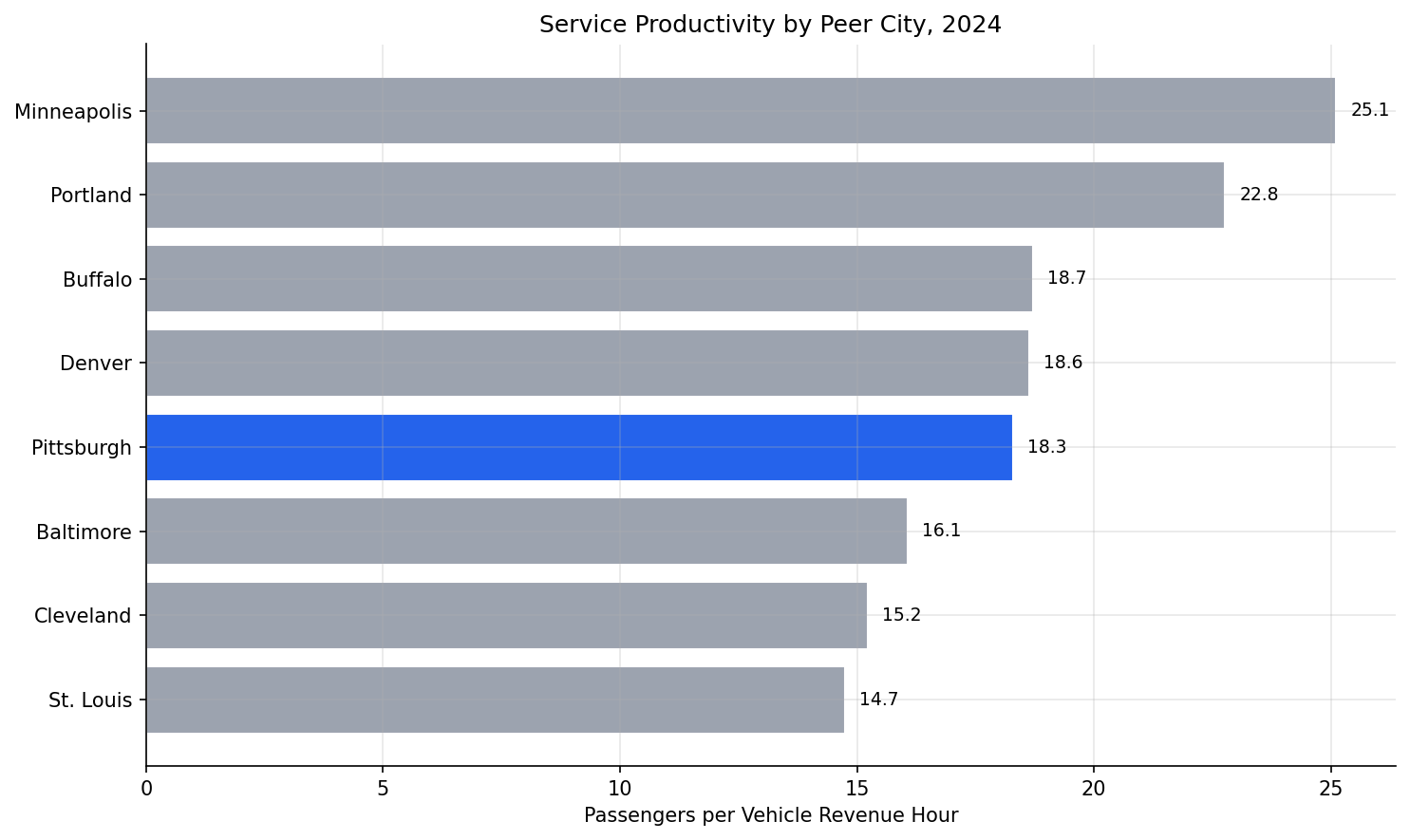
  • output/peer_productivity_2024.png — horizontal bar ranking of 2024 productivity across the 8 peers, PRT highlighted.
  • output/peer_productivity_trends.png — productivity trajectories 1991–2024 for all 8 peers, PRT highlighted.
  • output/per_capita_decomposition.csv — Allegheny County population, PRT UPT, VRH, productivity, and ridership per resident at 1991, 2000, 2010, 2020, 2024.
  • output/per_capita_normalization.png — county population, total ridership, and ridership per resident indexed to 1991 = 100.

Source Code

"""Analysis 48: tracks PRT service productivity (passengers per vehicle revenue
hour) from 1991 to 2024 and benchmarks it against peer cities."""

import math

import polars as pl

from prt_otp_analysis.common import (
    COLOR_GRAY,
    COLOR_PRIMARY,
    PEERS,
    analysis_dir,
    get_db,
    phase,
    run_analysis,
    save_chart,
    save_csv,
    setup_plotting,
)
from prt_otp_analysis.common.schemas import NTD_ANNUAL_SERVICE, validate

OUT = analysis_dir(__file__)

PRT_NTD_ID = 30022
START_YEAR = 1991
COVID_YEAR = 2020
BASELINE_YEAR = 2019
COMPARE_YEAR = 2024

# ntd_annual_service started including ACCESS paratransit (DR mode) in its VRH
# aggregate beginning in 2008. Pre-2008 figures are fixed-route only. To keep
# the PRT long-run trend on a consistent fixed-route basis, DR UPT and VRH are
# subtracted from the aggregate for years >= this cutoff.
ACCESS_CORRECTION_YEAR = 2008

# Allegheny County resident population -- PRT's service area. Decennial U.S.
# Census counts (1990-2020) plus the Census Bureau's Vintage 2024 Population
# Estimates Program figure (2020 census base of 1,250,578 less the reported
# 18,769 decline over 2020-2024). Used to normalize ridership per resident.
COUNTY_POPULATION = {
    1990: 1_336_449,
    2000: 1_281_666,
    2010: 1_223_348,
    2020: 1_250_578,
    2024: 1_231_809,
}
# The productivity record starts in 1991; the nearest decennial count is the
# 1990 census, used as the 1991 population anchor (a ~9-month offset).
POP_ANCHOR_YEARS = {1991: 1990, 2000: 2000, 2010: 2010, 2020: 2020, 2024: 2024}


def load_peer_productivity() -> pl.DataFrame:
    """Load annual UPT and VRH for all peer cities and derive productivity.

    Productivity is unlinked passenger trips per vehicle revenue hour
    (UPT / VRH) -- how many riders each hour of service carried.
    Uses ntd_annual_service (agency-wide, all modes) for consistency across
    agencies in the peer comparison.
    """
    id_list = ",".join(str(i) for i in PEERS)
    df = query_ntd(f"""
        SELECT ntd_id, year, upt, vrh
        FROM ntd_annual_service
        WHERE ntd_id IN ({id_list})
        ORDER BY ntd_id, year
    """)
    peer_map = pl.DataFrame({
        "ntd_id": list(PEERS.keys()),
        "city": list(PEERS.values()),
    })
    df = df.join(peer_map, on="ntd_id", how="left")
    return df.with_columns(productivity=(pl.col("upt") / pl.col("vrh")))


def load_prt_fixed_route() -> pl.DataFrame:
    """Build a consistent fixed-route UPT/VRH series for PRT, 1991-2024.

    ntd_annual_service excluded ACCESS (DR mode) from VRH before 2008, then
    started including it -- creating an artificial ~18% jump. For years >=
    ACCESS_CORRECTION_YEAR, DR UPT and VRH are subtracted from the aggregate
    using annual totals computed from ntd_ridership.
    Pre-2008 rows are taken from ntd_annual_service without adjustment (ACCESS
    was not in that aggregate).
    """
    conn = get_db()
    try:
        annual_rows = conn.execute("""
            SELECT year, upt, vrh
            FROM ntd_annual_service
            WHERE ntd_id = ?
            ORDER BY year
        """, (PRT_NTD_ID,)).fetchall()

        access_rows = conn.execute("""
            SELECT CAST(SUBSTR(month, 1, 4) AS INTEGER) AS year,
                   SUM(upt) AS dr_upt,
                   SUM(vrh) AS dr_vrh
            FROM ntd_ridership
            WHERE ntd_id = ? AND mode = 'DR'
            GROUP BY year
        """, (PRT_NTD_ID,)).fetchall()
    finally:
        conn.close()

    access_map: dict[int, tuple[float, float]] = {
        r[0]: (float(r[1] or 0), float(r[2] or 0)) for r in access_rows
    }

    rows = []
    for r in annual_rows:
        year, upt, vrh = r[0], float(r[1]), float(r[2])
        if year >= ACCESS_CORRECTION_YEAR:
            dr_upt, dr_vrh = access_map.get(year, (0.0, 0.0))
            upt -= dr_upt
            vrh -= dr_vrh
        rows.append({"year": year, "upt": upt, "vrh": vrh})

    df = pl.DataFrame(rows, schema={"year": pl.Int64, "upt": pl.Float64, "vrh": pl.Float64})
    return df.with_columns(productivity=pl.col("upt") / pl.col("vrh"))


def query_ntd(sql: str) -> pl.DataFrame:
    """Run a query against ntd_annual_service and validate the result schema."""
    conn = get_db()
    try:
        rows = conn.execute(sql).fetchall()
    finally:
        conn.close()
    df = pl.DataFrame(
        [dict(r) for r in rows],
        schema={"ntd_id": pl.Int64, "year": pl.Int64,
                "upt": pl.Float64, "vrh": pl.Float64},
    )
    return validate(df, NTD_ANNUAL_SERVICE, subset=True)


def chart_prt_trend(plt, prt_df: pl.DataFrame) -> None:
    """Line chart of PRT productivity across the full 1991-2024 record."""
    fig, ax = plt.subplots(figsize=(12, 6))
    years = prt_df["year"].to_list()
    vals = prt_df["productivity"].to_list()

    ax.plot(years, vals, color=COLOR_PRIMARY, linewidth=2.5, marker="o", markersize=4)
    ax.axvline(COVID_YEAR, color=COLOR_GRAY, linestyle="--", linewidth=1)
    ax.text(COVID_YEAR + 0.3, max(vals) * 0.97, "COVID-19", fontsize=9, color="#555555")

    first, last = vals[0], vals[-1]
    ax.annotate(f"{first:.1f}", (years[0], first), textcoords="offset points",
                xytext=(0, 10), ha="center", fontsize=9, fontweight="bold")
    ax.annotate(f"{last:.1f}", (years[-1], last), textcoords="offset points",
                xytext=(0, 10), ha="center", fontsize=9, fontweight="bold")

    ax.set_ylabel("Passengers per Vehicle Revenue Hour")
    ax.set_xlabel("Year")
    ax.set_ylim(bottom=0)
    ax.set_title("PRT Service Productivity, 1991–2024")
    save_chart(fig, OUT / "prt_productivity_trend.png")


def chart_decomposition(plt, prt_df: pl.DataFrame) -> None:
    """Index ridership, service hours, and productivity to 1991 = 100.

    Separates the two halves of the productivity ratio: if VRH (supply) holds
    flat while UPT (demand) collapses, the decline is empty buses, not a
    deliberate right-sizing of service.
    """
    fig, ax = plt.subplots(figsize=(12, 6))
    years = prt_df["year"].to_list()

    for col, label, color, lw in [
        ("vrh", "Service hours (VRH)", "#6ACC65", 2.0),
        ("upt", "Ridership (UPT)", "#4878CF", 2.0),
        ("productivity", "Productivity (UPT/VRH)", COLOR_PRIMARY, 2.8),
    ]:
        vals = prt_df[col].to_list()
        base = vals[0]
        ax.plot(years, [v / base * 100 for v in vals], label=label,
                color=color, linewidth=lw, marker="o", markersize=3)

    ax.axhline(100, color=COLOR_GRAY, linestyle=":", linewidth=0.8)
    ax.set_ylabel("Indexed to 1991 = 100")
    ax.set_xlabel("Year")
    ax.set_title("PRT Ridership vs. Service Hours — Why Productivity Fell")
    ax.legend()
    save_chart(fig, OUT / "supply_vs_demand_decomposition.png")


def chart_peer_2024(plt, peer_df: pl.DataFrame) -> None:
    """Bar chart ranking peer cities by 2024 productivity, PRT highlighted."""
    fig, ax = plt.subplots(figsize=(10, 6))
    snap_df = peer_df.filter(pl.col("year") == COMPARE_YEAR).sort("productivity")
    cities = snap_df["city"].to_list()
    vals = snap_df["productivity"].to_list()
    colors = [COLOR_PRIMARY if c == "Pittsburgh" else COLOR_GRAY for c in cities]

    ax.barh(cities, vals, color=colors, edgecolor="white")
    for i, v in enumerate(vals):
        ax.text(v + 0.3, i, f"{v:.1f}", va="center", fontsize=9)

    ax.set_xlabel("Passengers per Vehicle Revenue Hour")
    ax.set_title(f"Service Productivity by Peer City, {COMPARE_YEAR}")
    save_chart(fig, OUT / "peer_productivity_2024.png")


def chart_peer_trends(plt, peer_df: pl.DataFrame) -> None:
    """Line chart of productivity 1991-2024 for all peers, PRT highlighted."""
    fig, ax = plt.subplots(figsize=(12, 6))
    for city in sorted(PEERS.values()):
        city_df = peer_df.filter(pl.col("city") == city).sort("year")
        is_prt = city == "Pittsburgh"
        ax.plot(
            city_df["year"].to_list(), city_df["productivity"].to_list(),
            label=city,
            color=COLOR_PRIMARY if is_prt else None,
            linewidth=2.8 if is_prt else 1.2,
            alpha=1.0 if is_prt else 0.6,
            zorder=10 if is_prt else 1,
        )
    ax.set_ylabel("Passengers per Vehicle Revenue Hour")
    ax.set_xlabel("Year")
    ax.set_ylim(bottom=0)
    ax.set_title("Service Productivity — Pittsburgh vs. 7 Peer Cities, 1991–2024")
    ax.legend(fontsize=8, ncol=2)
    save_chart(fig, OUT / "peer_productivity_trends.png")


def peer_change_table(peer_df: pl.DataFrame) -> pl.DataFrame:
    """Wide table of productivity at 1991, 2019, and 2024 with percent changes."""
    keep = peer_df.filter(pl.col("year").is_in([START_YEAR, BASELINE_YEAR, COMPARE_YEAR]))
    wide = keep.pivot(values="productivity", index="city", on="year")
    wide = wide.rename({str(START_YEAR): "prod_1991",
                        str(BASELINE_YEAR): "prod_2019",
                        str(COMPARE_YEAR): "prod_2024"})
    return wide.with_columns(
        pct_change_1991_2024=((pl.col("prod_2024") - pl.col("prod_1991"))
                              / pl.col("prod_1991") * 100),
        pct_change_2019_2024=((pl.col("prod_2024") - pl.col("prod_2019"))
                              / pl.col("prod_2019") * 100),
    ).sort("prod_2024", descending=True)


def per_capita_decomposition(prt_df: pl.DataFrame) -> pl.DataFrame:
    """Normalize PRT ridership by Allegheny County population.

    Pairs each census/estimate year with the matching year in the NTD
    productivity record and derives ridership per resident (UPT / population).
    This splits the ridership decline into a population component (fewer
    residents) and a per-capita-usage component (each resident riding less).
    """
    rows = []
    for ntd_year, pop_year in POP_ANCHOR_YEARS.items():
        r = prt_df.filter(pl.col("year") == ntd_year).row(0, named=True)
        pop = COUNTY_POPULATION[pop_year]
        rows.append({
            "year": ntd_year,
            "population": pop,
            "upt": r["upt"],
            "vrh": r["vrh"],
            "productivity": r["productivity"],
            "trips_per_capita": r["upt"] / pop,
        })
    return pl.DataFrame(rows)


def chart_per_capita(plt, norm_df: pl.DataFrame) -> None:
    """Index population, total ridership, and per-capita ridership to 1991 = 100.

    Shows that PRT's ridership collapse is overwhelmingly fewer trips per
    resident, not fewer residents: county population barely moved while
    ridership per resident roughly halved.
    """
    fig, ax = plt.subplots(figsize=(12, 6))
    years = norm_df["year"].to_list()

    for col, label, color, lw in [
        ("population", "Allegheny County population", "#6ACC65", 2.0),
        ("upt", "Total ridership (UPT)", "#4878CF", 2.0),
        ("trips_per_capita", "Ridership per resident", COLOR_PRIMARY, 2.8),
    ]:
        vals = norm_df[col].to_list()
        base = vals[0]
        ax.plot(years, [v / base * 100 for v in vals], label=label,
                color=color, linewidth=lw, marker="o", markersize=6)

    ax.axhline(100, color=COLOR_GRAY, linestyle=":", linewidth=0.8)
    ax.set_ylabel("Indexed to 1991 = 100")
    ax.set_xlabel("Year")
    ax.set_ylim(bottom=0)
    ax.set_title("PRT Ridership per Resident vs. Population — Allegheny County")
    ax.legend()
    save_chart(fig, OUT / "per_capita_normalization.png")


@run_analysis(48, "Service Productivity")
def main():
    plt = setup_plotting()

    with phase("Loading NTD productivity data"):
        peer_df = load_peer_productivity()
        # Fixed-route-only series for PRT trend/decomposition charts. Peer
        # comparison charts use peer_df (agency-wide ntd_annual_service),
        # which is consistent across agencies for comparison purposes.
        prt_df = load_prt_fixed_route()
        print(f"   {len(peer_df)} city-years across {peer_df['city'].n_unique()} agencies")
        print(f"   PRT record: {prt_df['year'].min()}–{prt_df['year'].max()}")

    with phase("Summarizing PRT trajectory"):
        first = prt_df.row(0, named=True)
        last = prt_df.row(-1, named=True)
        drop = (last["productivity"] - first["productivity"]) / first["productivity"] * 100
        print(f"   {first['year']}: {first['productivity']:.1f} pax/VRH")
        print(f"   {last['year']}: {last['productivity']:.1f} pax/VRH  ({drop:+.0f}%)")
        vrh_chg = (last["vrh"] - first["vrh"]) / first["vrh"] * 100
        upt_chg = (last["upt"] - first["upt"]) / first["upt"] * 100
        print(f"   over the period: VRH {vrh_chg:+.0f}%, UPT {upt_chg:+.0f}%")

    with phase("Computing peer change table"):
        change_df = peer_change_table(peer_df)
        print(f"\n   {'City':<14s} {'1991':>7s} {'2019':>7s} {'2024':>7s} "
              f"{'91→24':>9s} {'19→24':>9s}")
        for r in change_df.iter_rows(named=True):
            mark = " <<<" if r["city"] == "Pittsburgh" else ""
            print("   %-14s %7.1f %7.1f %7.1f %+8.0f%% %+8.0f%%%s" % (
                r["city"], r["prod_1991"], r["prod_2019"], r["prod_2024"],
                r["pct_change_1991_2024"], r["pct_change_2019_2024"], mark))

    with phase("Normalizing ridership by population"):
        norm_df = per_capita_decomposition(prt_df)
        base = norm_df.row(0, named=True)
        end = norm_df.row(-1, named=True)
        pop_ratio = end["population"] / base["population"]
        upt_ratio = end["upt"] / base["upt"]
        pc_ratio = end["trips_per_capita"] / base["trips_per_capita"]
        # Multiplicative decomposition: UPT = population x trips-per-capita.
        # Log shares partition the ridership decline between the two factors.
        pop_share = math.log(pop_ratio) / math.log(upt_ratio)
        pc_share = math.log(pc_ratio) / math.log(upt_ratio)
        print(f"   Allegheny County population {base['year']}: "
              f"{base['population']:,} (1990 census)")
        print(f"   Allegheny County population {end['year']}: "
              f"{end['population']:,}  ({(pop_ratio - 1) * 100:+.0f}%)")
        print(f"   ridership per resident: {base['trips_per_capita']:.1f} → "
              f"{end['trips_per_capita']:.1f} trips/resident/yr  "
              f"({(pc_ratio - 1) * 100:+.0f}%)")
        print(f"   share of ridership decline from population loss: "
              f"{pop_share * 100:.0f}%")
        print(f"   share of ridership decline from lower per-capita use: "
              f"{pc_share * 100:.0f}%")

    with phase("Saving data"):
        save_csv(prt_df.select("year", "upt", "vrh", "productivity"),
                 OUT / "prt_productivity_by_year.csv")
        save_csv(change_df, OUT / "peer_productivity.csv")
        save_csv(norm_df, OUT / "per_capita_decomposition.csv")

    with phase("Generating charts"):
        chart_prt_trend(plt, prt_df)
        chart_decomposition(plt, prt_df)
        chart_peer_2024(plt, peer_df)
        chart_peer_trends(plt, peer_df)
        chart_per_capita(plt, norm_df)


if __name__ == "__main__":
    main()

Sources

NameTypeWhy It MattersOwnerFreshnessCaveat
ntd_annual_service table Primary analytical table used in this page's computations. Produced by NTD Annual Service ETL. Updated when the producing pipeline step is rerun. Coverage depends on upstream source availability and ETL assumptions.
Upstream sources (1)
  • file data/ntd-annual-service/2023_TS2.2_Service_Data.xlsx — NTD TS2.2 workbook with annual service data by system.
polars dependency Runtime dependency required for this page's pipeline or analysis code. Open-source Python ecosystem maintainers. Version pinned by project environment until dependency updates are applied. Library updates may change behavior or defaults.
matplotlib dependency Runtime dependency required for this page's pipeline or analysis code. Open-source Python ecosystem maintainers. Version pinned by project environment until dependency updates are applied. Library updates may change behavior or defaults.