Analysis

26 - Ridership in Multivariate OTP Model

Ridership and External Factors

Coverage: 2017-01 to 2025-11 (from otp_monthly, ridership_monthly).

Built 2026-03-03 02:23 UTC · Commit defd5c8

Page Navigation

Analysis Navigation

Data Provenance

flowchart LR
  26_ridership_multivariate(["26 - Ridership in Multivariate OTP Model"])
  t_otp_monthly[("otp_monthly")] --> 26_ridership_multivariate
  01_data_ingestion[["Data Ingestion"]] --> t_otp_monthly
  t_ridership_monthly[("ridership_monthly")] --> 26_ridership_multivariate
  01_data_ingestion[["Data Ingestion"]] --> t_ridership_monthly
  t_route_stops[("route_stops")] --> 26_ridership_multivariate
  01_data_ingestion[["Data Ingestion"]] --> t_route_stops
  t_routes[("routes")] --> 26_ridership_multivariate
  01_data_ingestion[["Data Ingestion"]] --> t_routes
  t_stops[("stops")] --> 26_ridership_multivariate
  01_data_ingestion[["Data Ingestion"]] --> t_stops
  d1_26_ridership_multivariate(("numpy (lib)")) --> 26_ridership_multivariate
  d2_26_ridership_multivariate(("polars (lib)")) --> 26_ridership_multivariate
  d3_26_ridership_multivariate(("scipy (lib)")) --> 26_ridership_multivariate
  classDef page fill:#dbeafe,stroke:#1d4ed8,color:#1e3a8a,stroke-width:2px;
  classDef table fill:#ecfeff,stroke:#0e7490,color:#164e63;
  classDef dep fill:#fff7ed,stroke:#c2410c,color:#7c2d12,stroke-dasharray: 4 2;
  classDef file fill:#eef2ff,stroke:#6366f1,color:#3730a3;
  classDef api fill:#f0fdf4,stroke:#16a34a,color:#14532d;
  classDef pipeline fill:#f5f3ff,stroke:#7c3aed,color:#4c1d95;
  class 26_ridership_multivariate page;
  class t_otp_monthly,t_ridership_monthly,t_route_stops,t_routes,t_stops table;
  class d1_26_ridership_multivariate,d2_26_ridership_multivariate,d3_26_ridership_multivariate dep;
  class 01_data_ingestion pipeline;

Findings

Findings: Ridership in Multivariate OTP Model

Summary

Adding log-transformed average weekday ridership to the Analysis 18 multivariate model does not significantly improve explanatory power. The F-test for the ridership term is not significant (F = 2.53, p = 0.116), and R² increases by only 1.5 pp (from 0.499 to 0.514). Ridership is not collinear with stop count or span (VIF = 1.73), but it is largely redundant with the existing predictors -- once route structure is controlled for, knowing how many people ride a route tells you almost nothing additional about its OTP.

Key Numbers

Model	R²	Adj R²	n
Base (6 features, Analysis 18 replication)	0.499	0.464	92
Expanded (+ log_riders)	0.514	0.473	92
Bus-only base (5 features)	0.392	0.355	89
Bus-only expanded (+ log_riders)	0.410	0.367	89
Ridership-only (log_riders + is_rail)	0.232	0.215	92

F-test for log_riders (all routes): F = 2.53, p = 0.116
F-test for log_riders (bus only): F = 2.55, p = 0.114
log_riders beta weight: -0.16 (weakly negative, not significant)
VIF for log_riders: 1.73 (no multicollinearity concern)
Ridership-only model explains just 23.2% of variance (vs 49.9% for structural model)

Expanded model coefficients

Feature	Beta Weight	p-value
stop_count	-0.43	<0.001
span_km	-0.47	<0.001
is_rail	+0.43	<0.001
n_munis	+0.35	0.005
log_riders	-0.16	0.116
is_premium_bus	+0.08	0.511
weekend_ratio	+0.06	0.605

Observations

The base model replicates Analysis 18's results closely (R² = 0.499 here vs 0.472 in Analysis 18; the small difference is because this analysis restricts to routes with ridership data, dropping 0 routes from the 92-route sample).
Log ridership has a weakly negative coefficient (beta = -0.16): higher-ridership routes tend to have slightly worse OTP after controls, but the effect is not statistically significant. This is consistent with Analysis 19's finding that ridership-weighted OTP is slightly higher than trip-weighted -- the two observations are not contradictory because the relationship is weak and confounded.
Log ridership is surprisingly uncorrelated with stop count (r = +0.15, p = 0.16) and span (r = -0.00, p = 1.00). It is most strongly correlated with weekend_ratio (r = +0.57) -- routes with more riders tend to have relatively more weekend service.
The ridership-only model (log_riders + is_rail, R² = 0.232) explains less than half the variance of the structural model (0.499), confirming that ridership is a weak proxy for the real drivers of OTP (stop count and span).
All VIFs remain below 3.0 in the expanded model, so multicollinearity is not a concern.

Discussion

This is a clean null result. Ridership does not add meaningful information to the OTP model once route structure is accounted for. The practical implication is that PRT does not need to worry that high ridership per se degrades OTP -- the routes with poor OTP happen to have high ridership because they are long, many-stop local bus corridors, not because passenger volumes cause delays. This is consistent with Analysis 10's finding that trip frequency does not predict OTP.

The weak negative direction of the ridership coefficient (-0.16 beta) is suggestive but not significant, and it could reflect residual confounding (high-ridership routes serve congested urban corridors) rather than a causal ridership-to-delay mechanism.

Caveats

Ridership is measured as average daily weekday riders per route, not per-trip load. Per-trip crowding data would better test the hypothesis that passenger volumes cause delays through dwell time.
The log transform assumes diminishing marginal effects; a linear specification also fails to reach significance (not shown).
The sample is restricted to 92 routes with both OTP and ridership data; 6 OTP-only routes are excluded.
As with Analysis 18, the model's unexplained 50% of variance likely requires operational data (traffic, staffing, schedule slack) not available in this dataset.

Output

image coefficient_comparison.png
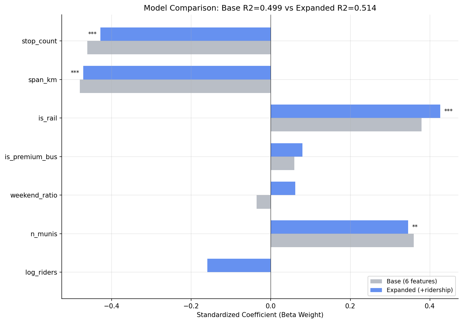
beta weight comparison between base and expanded models.

image partial_residual.png
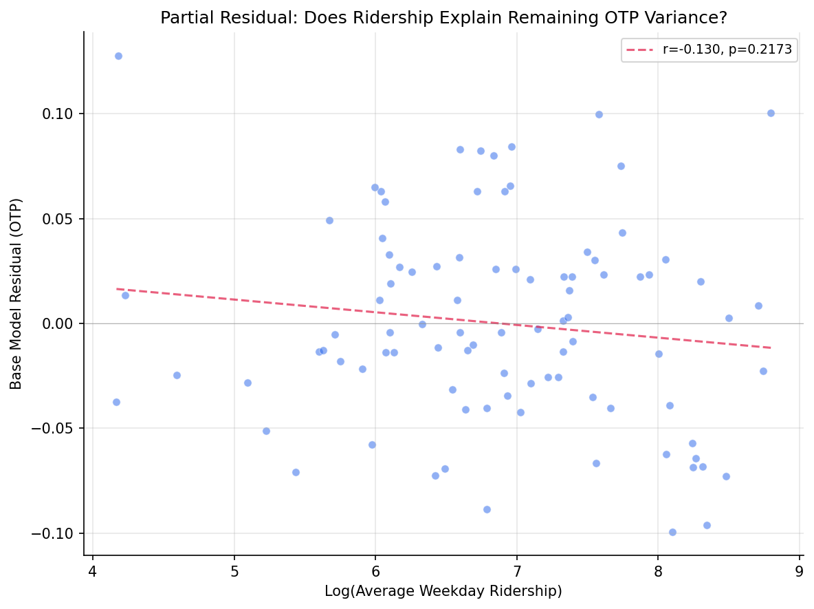
partial residual plot for log_ridership.

No interactive outputs declared.

data model_comparison.csv

side-by-side regression results (base vs expanded vs bus-only).

Preview CSV

Expand to load preview.

data vif_table.csv

VIF values for expanded model.

Preview CSV

Expand to load preview.

Methods

Methods: Ridership in Multivariate OTP Model

Question

Does average ridership add explanatory power to the Analysis 18 OLS model (stop count, span, mode, n_munis, premium, weekend ratio) or is it collinear with existing predictors?

Approach

Replicate the Analysis 18 six-feature OLS model on routes with ridership data available.
Add log-transformed average weekday ridership as a seventh predictor. Log transform is used because ridership is right-skewed and the relationship with OTP is expected to be diminishing (doubling from 100 to 200 riders matters more than from 5,000 to 5,100).
Compare adjusted R² between the six-feature and seven-feature models using a nested F-test.
Check VIF for the expanded model to assess multicollinearity with stop count and span.
If ridership is significant, test a reduced model (ridership + mode only) to see if ridership proxies for stop count.
Report beta weights, p-values, and model comparison statistics.
Repeat with bus-only subset.

Data

Name	Description	Source
`otp_monthly`	route_id, month, otp (averaged to route-level)	`prt.db` table
`ridership_monthly`	route_id, month, avg_riders (averaged across all months); filtered to day_type='WEEKDAY'	`prt.db` table
`route_stops`	route_id, stop_id for stop counts	`prt.db` table
`stops`	lat, lon for geographic span computation	`prt.db` table
`routes`	route_id, mode for subtype classification	`prt.db` table

Notes: Overlap period (Jan 2019 -- Oct 2024); exclude routes with fewer than 12 months of paired data.

Output

output/model_comparison.csv -- side-by-side regression results (base vs expanded vs bus-only)
output/vif_table.csv -- VIF values for expanded model
output/coefficient_comparison.png -- beta weight comparison between base and expanded models
output/partial_residual.png -- partial residual plot for log_ridership

Sources

Name	Type	Why It Matters	Owner	Freshness	Caveat
otp_monthly	table	Primary analytical table used in this page's computations.	Produced by Data Ingestion.	Updated when the producing pipeline step is rerun.	Coverage depends on upstream source availability and ETL assumptions.
ridership_monthly	table	Primary analytical table used in this page's computations.	Produced by Data Ingestion.	Updated when the producing pipeline step is rerun.	Coverage depends on upstream source availability and ETL assumptions.
route_stops	table	Primary analytical table used in this page's computations.	Produced by Data Ingestion.	Updated when the producing pipeline step is rerun.	Coverage depends on upstream source availability and ETL assumptions.
routes	table	Primary analytical table used in this page's computations.	Produced by Data Ingestion.	Updated when the producing pipeline step is rerun.	Coverage depends on upstream source availability and ETL assumptions.
stops	table	Primary analytical table used in this page's computations.	Produced by Data Ingestion.	Updated when the producing pipeline step is rerun.	Coverage depends on upstream source availability and ETL assumptions.
numpy	dependency	Runtime dependency required for this page's pipeline or analysis code.	Open-source Python ecosystem maintainers.	Version pinned by project environment until dependency updates are applied.	Library updates may change behavior or defaults.
polars	dependency	Runtime dependency required for this page's pipeline or analysis code.	Open-source Python ecosystem maintainers.	Version pinned by project environment until dependency updates are applied.	Library updates may change behavior or defaults.
scipy	dependency	Runtime dependency required for this page's pipeline or analysis code.	Open-source Python ecosystem maintainers.	Version pinned by project environment until dependency updates are applied.	Library updates may change behavior or defaults.