"""Analysis 24: Compare weekday, Saturday, and Sunday ridership trends and correlate weekend share with OTP."""

import polars as pl
from scipy import stats

from prt_otp_analysis.common import PRE_COVID_BASELINE_MONTH, analysis_dir, correlate, phase, query_to_polars, run_analysis, save_chart, save_csv, setup_plotting

OUT = analysis_dir(__file__)


def load_ridership() -> pl.DataFrame:
    """Load all ridership data across day types."""
    return query_to_polars("""
        SELECT route_id, month, day_type, avg_riders, day_count
        FROM ridership_monthly
        WHERE avg_riders IS NOT NULL AND day_count IS NOT NULL
    """)


def load_otp() -> pl.DataFrame:
    """Load OTP data for correlation analysis."""
    return query_to_polars("""
        SELECT route_id, month, otp
        FROM otp_monthly
    """)


def system_monthly(df: pl.DataFrame) -> pl.DataFrame:
    """Compute system-wide total monthly riders by day type."""
    return (
        df.with_columns(
            (pl.col("avg_riders") * pl.col("day_count")).alias("total_riders"),
        )
        .group_by("month", "day_type")
        .agg(
            total_riders=pl.col("total_riders").sum(),
            avg_riders_sum=pl.col("avg_riders").sum(),
            n_routes=pl.col("route_id").n_unique(),
        )
        .sort("month", "day_type")
    )


def index_to_baseline(monthly: pl.DataFrame, baseline_month: str = PRE_COVID_BASELINE_MONTH) -> pl.DataFrame:
    """Index each day type series to baseline_month = 100."""
    baseline = (
        monthly.filter(pl.col("month") == baseline_month)
        .select("day_type", pl.col("total_riders").alias("baseline_riders"))
    )
    return (
        monthly.join(baseline, on="day_type", how="left")
        .with_columns(
            (pl.col("total_riders") / pl.col("baseline_riders") * 100).alias("indexed"),
        )
    )


def weekend_share_monthly(monthly: pl.DataFrame) -> pl.DataFrame:
    """Compute weekend ridership share per month."""
    pivoted = (
        monthly.group_by("month")
        .agg(
            weekday=pl.col("total_riders").filter(pl.col("day_type") == "WEEKDAY").sum(),
            saturday=pl.col("total_riders").filter(pl.col("day_type") == "SAT.").sum(),
            sunday=pl.col("total_riders").filter(pl.col("day_type") == "SUN.").sum(),
        )
        .with_columns(
            total=pl.col("weekday") + pl.col("saturday") + pl.col("sunday"),
        )
        .with_columns(
            weekend_share=(pl.col("saturday") + pl.col("sunday")) / pl.col("total"),
            sat_share=pl.col("saturday") / pl.col("total"),
            sun_share=pl.col("sunday") / pl.col("total"),
        )
        .sort("month")
    )
    return pivoted


def route_weekend_share(df: pl.DataFrame) -> pl.DataFrame:
    """Compute per-route average weekend-to-weekday ridership ratio.

    For each route-month where all three day types are present, compute:
      weekend_ratio = (SAT avg_riders + SUN avg_riders) / WEEKDAY avg_riders
    Then average across months.
    """
    # Pivot to get all three day types per route-month
    wide = (
        df.pivot(on="day_type", index=["route_id", "month"], values="avg_riders")
    )
    # Only keep rows where all three day types are present
    required = ["WEEKDAY", "SAT.", "SUN."]
    for col in required:
        if col not in wide.columns:
            return pl.DataFrame()
    wide = wide.drop_nulls(subset=required)
    wide = wide.filter(pl.col("WEEKDAY") > 0)

    wide = wide.with_columns(
        weekend_ratio=(
            (pl.col("SAT.") + pl.col("SUN.")) / pl.col("WEEKDAY")
        ),
    )

    route_avg = (
        wide.group_by("route_id")
        .agg(
            avg_weekend_ratio=pl.col("weekend_ratio").mean(),
            n_months=pl.col("month").count(),
        )
        .filter(pl.col("n_months") >= 6)  # require at least 6 months with all day types
        .sort("avg_weekend_ratio", descending=True)
    )
    return route_avg


def correlate_weekend_otp(route_wkend: pl.DataFrame, otp_df: pl.DataFrame) -> dict:
    """Correlate route-level weekend share with average OTP."""
    if len(route_wkend) == 0:
        return {"n": 0, "error": "no routes with weekend data"}
    route_otp = (
        otp_df.group_by("route_id")
        .agg(avg_otp=pl.col("otp").mean())
    )
    merged = route_wkend.join(route_otp, on="route_id", how="inner")
    if len(merged) < 10:
        return {"n": len(merged), "error": "too few routes"}

    corr = correlate(merged, "avg_weekend_ratio", "avg_otp")

    return {
        "n": len(merged),
        "r_pearson": corr["pearson_r"],
        "p_pearson": corr["pearson_p"],
        "r_spearman": corr["spearman_r"],
        "p_spearman": corr["spearman_p"],
        "merged": merged,
    }


def make_trend_chart(monthly_idx: pl.DataFrame) -> None:
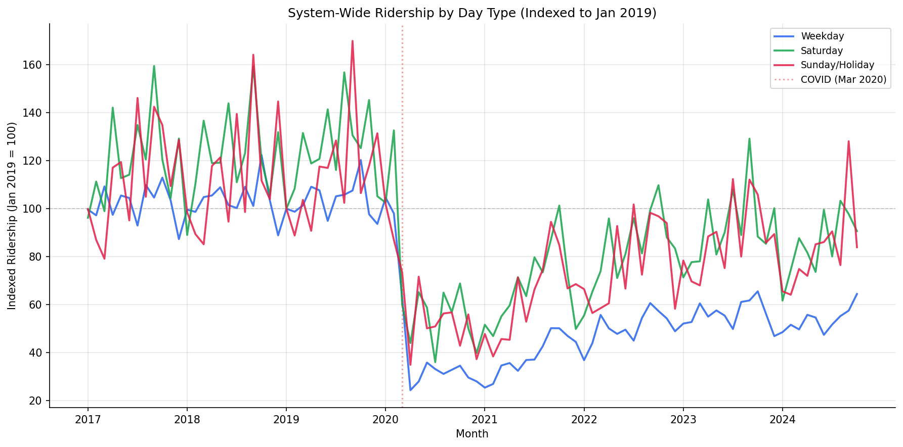
    """Plot indexed ridership by day type over time."""
    plt = setup_plotting()
    fig, ax = plt.subplots(figsize=(12, 6))

    day_type_styles = {
        "WEEKDAY": {"color": "#2563eb", "label": "Weekday"},
        "SAT.": {"color": "#16a34a", "label": "Saturday"},
        "SUN.": {"color": "#e11d48", "label": "Sunday/Holiday"},
    }

    all_months = sorted(monthly_idx["month"].unique().to_list())
    month_to_x = {m: i for i, m in enumerate(all_months)}
    tick_positions = [i for i, m in enumerate(all_months) if m.endswith("-01")]
    tick_labels = [all_months[i][:4] for i in tick_positions]

    for day_type, style in day_type_styles.items():
        sub = monthly_idx.filter(pl.col("day_type") == day_type).sort("month")
        if len(sub) == 0:
            continue
        x = [month_to_x[m] for m in sub["month"].to_list()]
        y = sub["indexed"].to_list()
        ax.plot(x, y, color=style["color"], linewidth=1.8, label=style["label"], alpha=0.85)

    ax.axhline(100, color="gray", linestyle="--", alpha=0.4, linewidth=0.8)

    if "2020-03" in all_months:
        covid_idx = month_to_x["2020-03"]
        ax.axvline(covid_idx, color="#ef4444", linestyle=":", alpha=0.5, label="COVID (Mar 2020)")

    ax.set_ylabel("Indexed Ridership (Jan 2019 = 100)")
    ax.set_xlabel("Month")
    ax.set_title("System-Wide Ridership by Day Type (Indexed to Jan 2019)")
    ax.set_xticks(tick_positions)
    ax.set_xticklabels(tick_labels)
    ax.legend(loc="upper right", fontsize=9)

    save_chart(fig, OUT / "daytype_ridership_trend.png")


def make_weekend_share_chart(wk_share: pl.DataFrame) -> None:
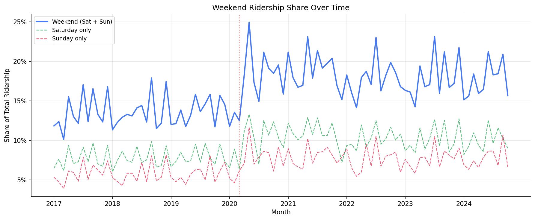
    """Plot weekend ridership share over time."""
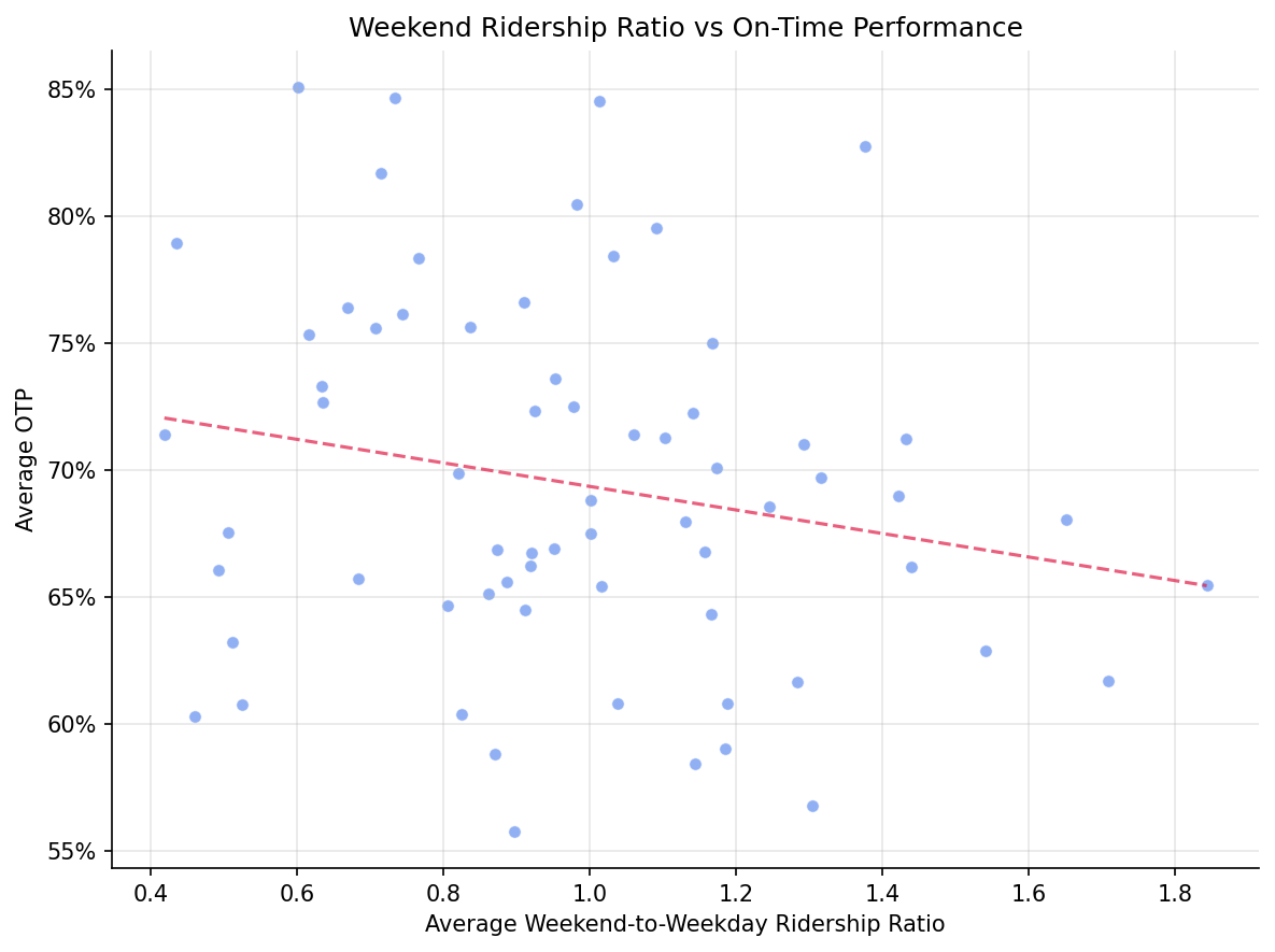
    plt = setup_plotting()
    fig, ax = plt.subplots(figsize=(12, 5))

    all_months = sorted(wk_share["month"].to_list())
    month_to_x = {m: i for i, m in enumerate(all_months)}
    tick_positions = [i for i, m in enumerate(all_months) if m.endswith("-01")]
    tick_labels = [all_months[i][:4] for i in tick_positions]

    x = [month_to_x[m] for m in wk_share["month"].to_list()]
    y_total = wk_share["weekend_share"].to_list()
    y_sat = wk_share["sat_share"].to_list()
    y_sun = wk_share["sun_share"].to_list()

    ax.plot(x, y_total, color="#2563eb", linewidth=2.0, label="Weekend (Sat + Sun)", alpha=0.85)
    ax.plot(x, y_sat, color="#16a34a", linewidth=1.2, label="Saturday only", alpha=0.7, linestyle="--")
    ax.plot(x, y_sun, color="#e11d48", linewidth=1.2, label="Sunday only", alpha=0.7, linestyle="--")

    if "2020-03" in all_months:
        covid_idx = month_to_x["2020-03"]
        ax.axvline(covid_idx, color="#ef4444", linestyle=":", alpha=0.5)

    ax.set_ylabel("Share of Total Ridership")
    ax.set_xlabel("Month")
    ax.set_title("Weekend Ridership Share Over Time")
    ax.set_xticks(tick_positions)
    ax.set_xticklabels(tick_labels)
    ax.legend(loc="upper left", fontsize=9)
    ax.yaxis.set_major_formatter(plt.FuncFormatter(lambda v, _: f"{v:.0%}"))

    save_chart(fig, OUT / "weekend_share_trend.png")


def make_scatter_chart(merged: pl.DataFrame) -> None:
    """Scatter plot of weekend ratio vs route-level OTP."""
    plt = setup_plotting()
    fig, ax = plt.subplots(figsize=(8, 6))

    x = merged["avg_weekend_ratio"].to_list()
    y = merged["avg_otp"].to_list()

    ax.scatter(x, y, alpha=0.5, s=30, color="#2563eb", edgecolors="white", linewidth=0.5)

    # Trend line
    slope, intercept, _, _, _ = stats.linregress(x, y)
    x_line = [min(x), max(x)]
    y_line = [slope * xi + intercept for xi in x_line]
    ax.plot(x_line, y_line, color="#e11d48", linewidth=1.5, linestyle="--", alpha=0.7)

    ax.set_xlabel("Average Weekend-to-Weekday Ridership Ratio")
    ax.set_ylabel("Average OTP")
    ax.set_title("Weekend Ridership Ratio vs On-Time Performance")
    ax.yaxis.set_major_formatter(plt.FuncFormatter(lambda v, _: f"{v:.0%}"))

    save_chart(fig, OUT / "weekend_share_vs_otp.png")


@run_analysis(24, "Weekday vs Weekend Ridership Trends")
def main() -> None:
    """Entry point: load data, compute trends, correlate, chart, and save."""

    with phase("Loading ridership data"):
        ride_df = load_ridership()
        print(f"  {len(ride_df):,} rows, {ride_df['route_id'].n_unique()} routes, "
              f"{ride_df['day_type'].n_unique()} day types")
        print(f"  Day types: {sorted(ride_df['day_type'].unique().to_list())}")
        print(f"  Month range: {ride_df['month'].min()} to {ride_df['month'].max()}")

    with phase("Computing system-wide monthly ridership by day type"):
        monthly = system_monthly(ride_df)

        # Summary stats by day type
        print("\n  Day type summary (total monthly riders, averaged across months):")
        for dt in sorted(monthly["day_type"].unique().to_list()):
            sub = monthly.filter(pl.col("day_type") == dt)
            avg = sub["total_riders"].mean()
            print(f"    {dt:<12s}: {avg:>12,.0f} avg monthly riders")

    with phase("Indexing to Jan 2019 baseline"):
        monthly_idx = index_to_baseline(monthly, PRE_COVID_BASELINE_MONTH)

        # Latest index values
        latest_month = monthly_idx["month"].max()
        print(f"\n  Latest month ({latest_month}) indexed values:")
        latest = monthly_idx.filter(pl.col("month") == latest_month)
        for row in latest.iter_rows(named=True):
            print(f"    {row['day_type']:<12s}: {row['indexed']:>6.1f}")

    with phase("Computing weekend ridership share"):
        wk_share = weekend_share_monthly(monthly)

        # Pre-COVID vs latest weekend share
        pre_covid_avg = wk_share.filter(
            (pl.col("month") >= PRE_COVID_BASELINE_MONTH) & (pl.col("month") <= "2020-02")
        )["weekend_share"].mean()
        post_2023_avg = wk_share.filter(pl.col("month") >= "2023-01")["weekend_share"].mean()
        print(f"\n  Weekend share (pre-COVID, 2019-01 to 2020-02): {pre_covid_avg:.1%}")
        print(f"  Weekend share (2023-01 to latest):             {post_2023_avg:.1%}")
        print(f"  Change: {post_2023_avg - pre_covid_avg:+.1%}")

    with phase("Computing per-route weekend-to-weekday ratio"):
        route_wkend = route_weekend_share(ride_df)
        print(f"  {len(route_wkend)} routes with 6+ months of all three day types")

        if len(route_wkend) > 0:
            print(f"  Median weekend ratio: {route_wkend['avg_weekend_ratio'].median():.3f}")
            print(f"  Range: {route_wkend['avg_weekend_ratio'].min():.3f} -- "
                  f"{route_wkend['avg_weekend_ratio'].max():.3f}")

            # Top/bottom 5
            print("\n  Top 5 weekend-heavy routes:")
            for row in route_wkend.head(5).iter_rows(named=True):
                print(f"    {row['route_id']:<8s} ratio={row['avg_weekend_ratio']:.3f}")
            print("  Bottom 5 weekend-heavy routes:")
            for row in route_wkend.tail(5).iter_rows(named=True):
                print(f"    {row['route_id']:<8s} ratio={row['avg_weekend_ratio']:.3f}")

    with phase("Correlating weekend share with OTP"):
        otp_df = load_otp()
        corr = correlate_weekend_otp(route_wkend, otp_df)
        if "error" not in corr:
            print(f"  n = {corr['n']} routes")
            print(f"  Pearson  r = {corr['r_pearson']:.3f}, p = {corr['p_pearson']:.4f}")
            print(f"  Spearman r = {corr['r_spearman']:.3f}, p = {corr['p_spearman']:.4f}")
        else:
            print(f"  {corr['error']}")

    with phase("Saving CSV"):
        save_csv(monthly, OUT / "daytype_summary.csv")

    with phase("Generating charts"):
        make_trend_chart(monthly_idx)
        make_weekend_share_chart(wk_share)
        if "merged" in corr:
            make_scatter_chart(corr["merged"])


if __name__ == "__main__":
    main()