Analysis

17: Weekend vs Weekday Service Profile

Route and Service Drivers

Coverage: 2019-01 to 2025-11 (from otp_monthly).

Built 2026-03-03 02:23 UTC · Commit defd5c8

Page Navigation

Analysis Navigation

Data Provenance

flowchart LR
  17_weekend_weekday_profile(["17: Weekend vs Weekday Service Profile"])
  t_otp_monthly[("otp_monthly")] --> 17_weekend_weekday_profile
  01_data_ingestion[["Data Ingestion"]] --> t_otp_monthly
  t_route_stops[("route_stops")] --> 17_weekend_weekday_profile
  01_data_ingestion[["Data Ingestion"]] --> t_route_stops
  t_routes[("routes")] --> 17_weekend_weekday_profile
  01_data_ingestion[["Data Ingestion"]] --> t_routes
  d1_17_weekend_weekday_profile(("polars (lib)")) --> 17_weekend_weekday_profile
  d2_17_weekend_weekday_profile(("scipy (lib)")) --> 17_weekend_weekday_profile
  classDef page fill:#dbeafe,stroke:#1d4ed8,color:#1e3a8a,stroke-width:2px;
  classDef table fill:#ecfeff,stroke:#0e7490,color:#164e63;
  classDef dep fill:#fff7ed,stroke:#c2410c,color:#7c2d12,stroke-dasharray: 4 2;
  classDef file fill:#eef2ff,stroke:#6366f1,color:#3730a3;
  classDef api fill:#f0fdf4,stroke:#16a34a,color:#14532d;
  classDef pipeline fill:#f5f3ff,stroke:#7c3aed,color:#4c1d95;
  class 17_weekend_weekday_profile page;
  class t_otp_monthly,t_route_stops,t_routes table;
  class d1_17_weekend_weekday_profile,d2_17_weekend_weekday_profile dep;
  class 01_data_ingestion pipeline;

Findings

Findings: Weekend vs Weekday Service Profile

Summary

There is no meaningful correlation between a route's weekend-to-weekday service ratio and its OTP. Routes that run heavy weekend service perform identically to commuter-oriented weekday-heavy routes.

Key Numbers

Pearson r = -0.03 (p = 0.79, n = 93)
Spearman rho = -0.02 (p = 0.84)

Service Tier	Routes	Mean OTP
Weekday-heavy (<0.3)	27	69.8%
Balanced (0.3-0.7)	45	68.8%
Weekend-heavy (>0.7)	21	70.3%

Observations

The three service tiers are virtually indistinguishable in OTP (69.8%, 68.8%, 70.3%).
Neither Pearson nor Spearman correlations approach significance.
This null result makes sense: the weekend service ratio reflects demand patterns and scheduling choices, not route structure. A route with high weekend service isn't inherently harder to run on time.
Since OTP is reported monthly (not by day-of-week), it aggregates weekday and weekend performance, which may mask day-specific patterns.
Bus-only correlation (r = -0.06, p = 0.56) confirms the null result holds within the dominant mode.

Implication

Weekend vs weekday service intensity is not a useful predictor of OTP. The structural factors identified in other analyses (stop count, mode, route length) dominate.

Review History

2026-02-10: RED-TEAM-REPORTS/2026-02-10-analyses-12-18.md — 2 issues (both moderate). Bus-only correlation added; caveats strengthened. Null finding unchanged.

Output

image service_tier_comparison.png
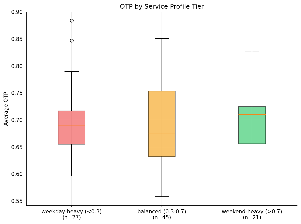
box plot by service profile tier.

image weekend_ratio_vs_otp.png
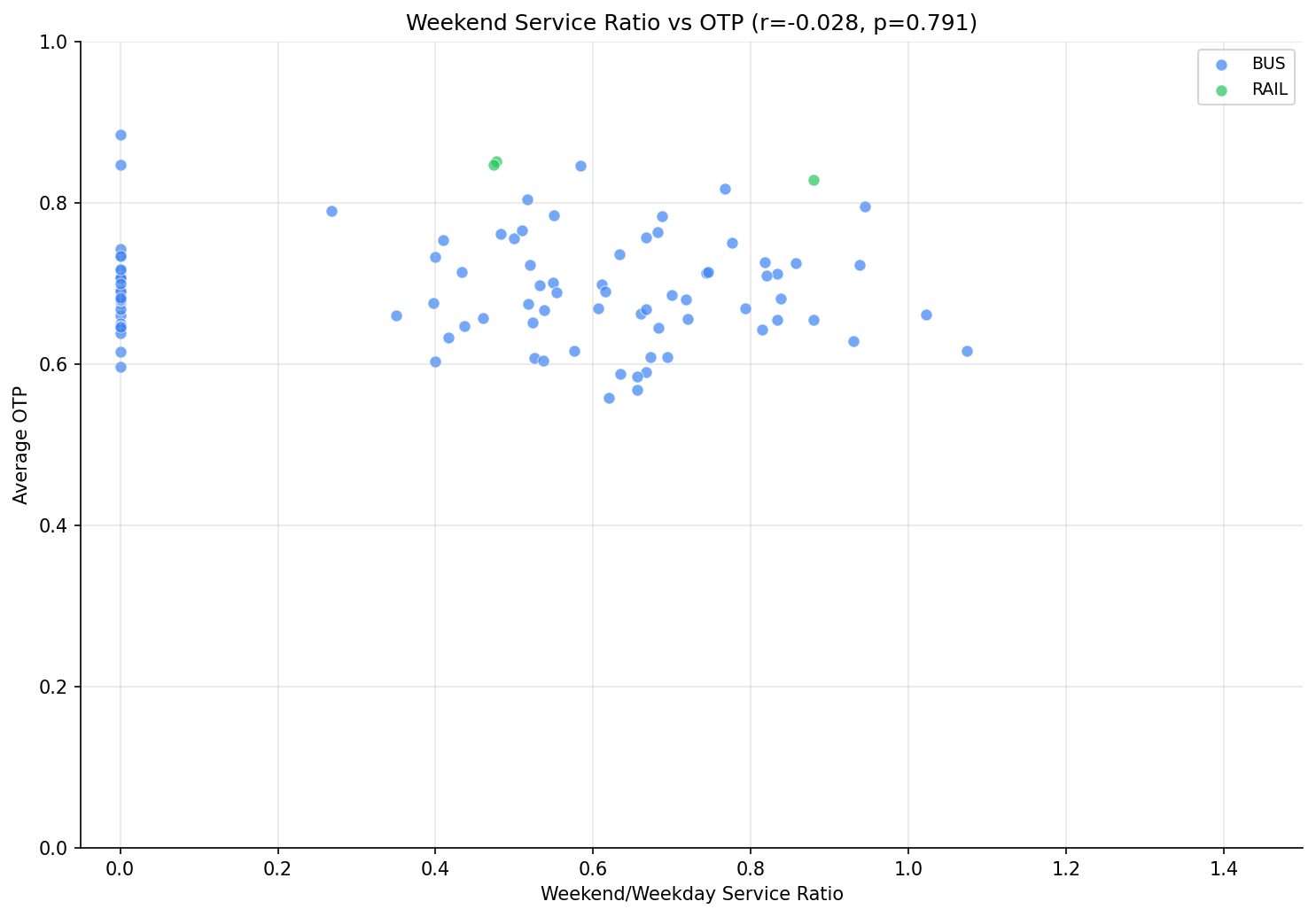
scatter plot.

No interactive outputs declared.

data service_profile.csv

per-route trip counts, weekend ratio, and OTP.

Preview CSV

Expand to load preview.

Methods

Methods: Weekend vs Weekday Service Profile

Question

Do commuter-oriented routes (high weekday, low weekend service) perform differently than all-day routes (similar weekday and weekend service)? The ratio of weekend to weekday trips signals route purpose, and since OTP is reported monthly, it likely reflects weekday-dominant measurement.

Approach

For each route, compute peak weekday trips (MAX trips_wd), peak Saturday trips (MAX trips_sa), and peak Sunday trips (MAX trips_su) from route_stops.
Compute weekend ratio = (max_sa + max_su) / (2 * max_wd), representing the proportion of weekday service provided on weekends (1.0 = identical, 0 = weekday-only).
Correlate weekend ratio with average OTP.
Classify routes as weekday-heavy (ratio < 0.3), balanced (0.3-0.7), or weekend-heavy (> 0.7) and compare OTP distributions.
Scatter plot and box plot.

Data

Name	Description	Source
`route_stops`	Weekday, Saturday, Sunday trip counts per stop	`prt.db` table
`otp_monthly`	Monthly OTP per route	`prt.db` table
`routes`	Mode and name	`prt.db` table

Output

output/service_profile.csv -- per-route trip counts, weekend ratio, and OTP
output/weekend_ratio_vs_otp.png -- scatter plot
output/service_tier_comparison.png -- box plot by service profile tier

Sources

Name	Type	Why It Matters	Owner	Freshness	Caveat
otp_monthly	table	Primary analytical table used in this page's computations.	Produced by Data Ingestion.	Updated when the producing pipeline step is rerun.	Coverage depends on upstream source availability and ETL assumptions.
route_stops	table	Primary analytical table used in this page's computations.	Produced by Data Ingestion.	Updated when the producing pipeline step is rerun.	Coverage depends on upstream source availability and ETL assumptions.
routes	table	Primary analytical table used in this page's computations.	Produced by Data Ingestion.	Updated when the producing pipeline step is rerun.	Coverage depends on upstream source availability and ETL assumptions.
polars	dependency	Runtime dependency required for this page's pipeline or analysis code.	Open-source Python ecosystem maintainers.	Version pinned by project environment until dependency updates are applied.	Library updates may change behavior or defaults.
scipy	dependency	Runtime dependency required for this page's pipeline or analysis code.	Open-source Python ecosystem maintainers.	Version pinned by project environment until dependency updates are applied.	Library updates may change behavior or defaults.