Findings: Municipal/County Equity

Summary

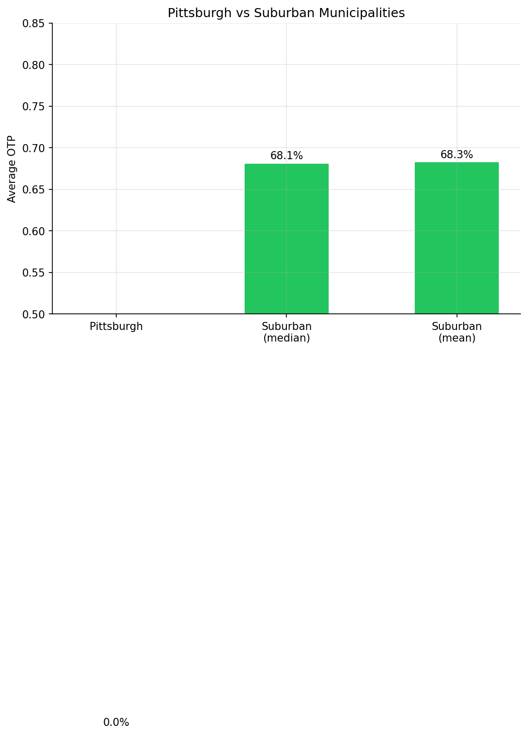
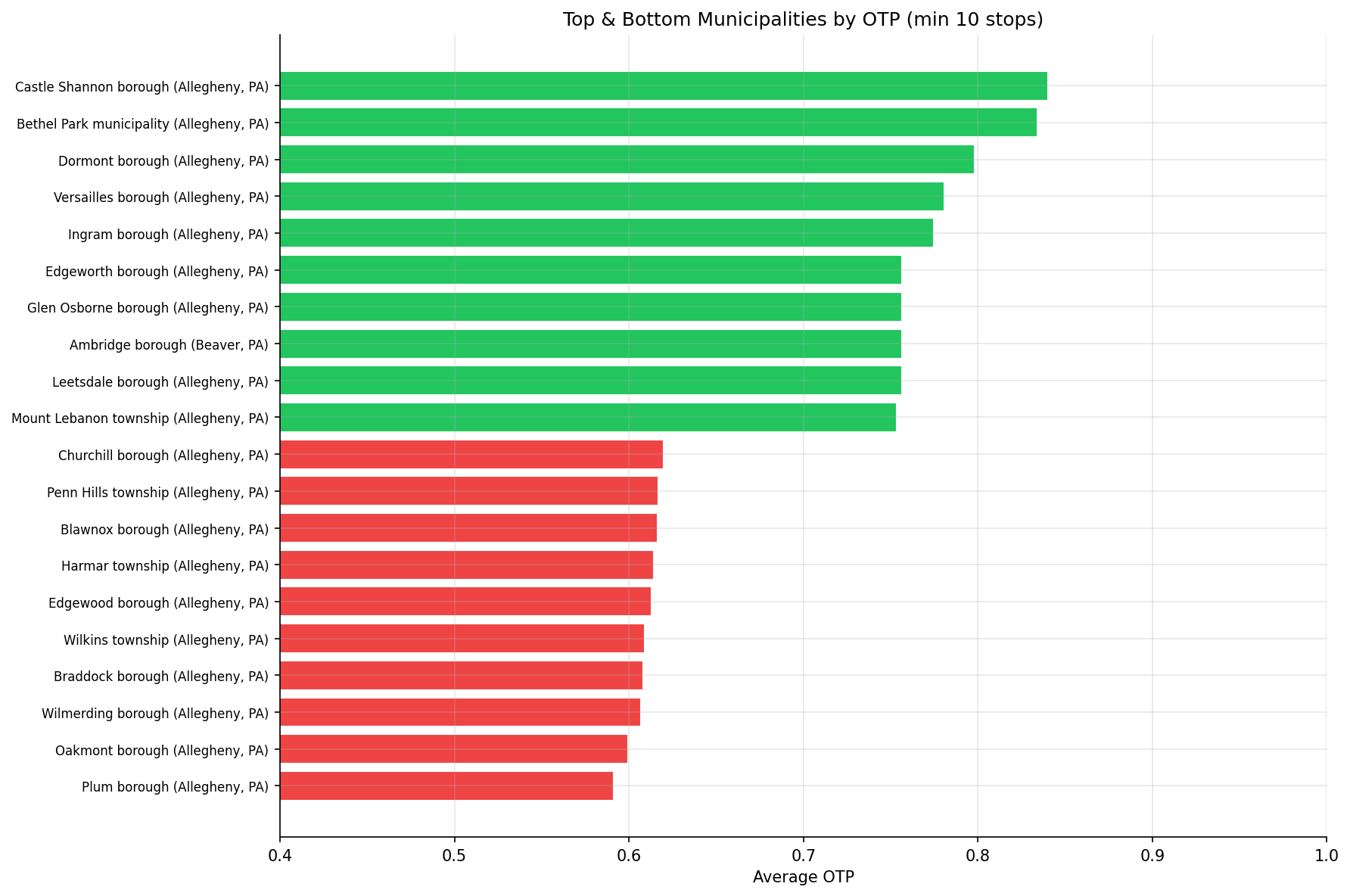
81 municipalities had enough stops (10+) to analyze. There is a 25 pp spread between the best and worst municipalities, similar to the neighborhood-level equity gap. Cross-jurisdictional routes (serving 2+ municipalities) perform no differently from single-municipality routes.

Key Numbers

• 81 municipalities analyzed (with much better data coverage than the 89 neighborhoods in Analysis 04)
• Best: Castle Shannon borough (84.0%)
• Worst: Plum borough (59.1%)
• Spread: 24.9 pp
• Suburban median OTP: 68.1%
• Cross-jurisdictional routes (n=74): avg OTP = 69.5%
• Single-municipality routes (n=19): avg OTP = 69.2%
• Cross vs single t-test: p = 0.85 -- no significant difference

Observations

• The best-performing municipalities (Castle Shannon, Dormont, Beechview) are all served by the light rail T line, consistent with the mode advantage found in Analysis 02.
• The worst-performing municipalities (Plum, Penn Hills, Wilkinsburg) are served primarily by long local bus routes through the eastern corridor.
• The suburban median OTP (68.1%) is very close to the overall system average, suggesting no systematic suburban vs urban disadvantage.
• Cross-jurisdictional routes -- which might be expected to suffer from longer distances and more complexity -- perform identically to single-municipality routes. Route length and stop count matter more than jurisdictional boundaries.
• The municipal analysis has much better data coverage than the neighborhood analysis (Analysis 04), which lost 58% of stops due to missing hood data.

Implication

The equity gap is driven by mode and route structure, not by geography per se. Municipalities on rail or busway corridors get 80%+ OTP; those served only by long local bus routes get 60%. Municipal boundaries and suburban/urban distinctions are not meaningful predictors.

Caveats

• Route OTP is projected onto stops and then onto municipalities (ecological fallacy). A route's performance may vary along its length, and municipalities at the ends of long routes may experience different OTP than those near the middle.
• Trip weights (trips_7d) are a static snapshot applied across the full study period. Service levels changed over time, especially during COVID.

Review History

• 2026-02-10: RED-TEAM-REPORTS/2026-02-10-analyses-12-18.md — 3 issues (2 significant, inherent to data). Ecological fallacy documented; Welch's t-test applied (no material change).

Methods: Municipal/County Equity

Question

Analysis 04 examined neighborhood equity but lost 58% of stops due to missing hood data. The muni (municipality) and county fields have broader coverage. Do suburban municipalities get better or worse service reliability than the City of Pittsburgh? Do routes that cross municipal boundaries perform differently?

Approach

• For each stop, assign OTP from the routes serving it (trip-weighted average from route_stops and otp_monthly).
• Aggregate stop-level OTP by municipality and county, weighted by trips.
• Rank municipalities by average OTP.
• Identify cross-jurisdictional routes (routes with stops in 2+ municipalities) and compare their OTP to single-municipality routes.
• Compare Pittsburgh city vs suburban municipalities.
• Bar chart of top/bottom municipalities, and Pittsburgh vs suburban comparison.

Data

Output

• output/municipal_otp.csv -- per-municipality average OTP and stop count
• output/top_bottom_municipalities.png -- bar chart of best/worst municipalities
• output/pittsburgh_vs_suburban.png -- comparison chart